1 Objectives

Explore the calculation of maximum likelihood;
Perform the log-likelihood ratio test;
Evaluate statistical results for likelihood test;
Practice graphical display of likelihood problems.

2 Start a Script

For this lab or project, begin by:

Starting a new R script
Create a good header section and table of contents
Save the script file with an informative name
set your working directory

Aim to make the script a future reference for doing things in R!

3 Introduction

In this lab we will use likelihood methods to estimate parameters and test hypotheses. Likelihood methods are especially useful when modeling data having a probability distribution other than the normal distribution (e.g., binomial, exponential, etc).

3.1 Maximum likelihood estimate

To estimate a parameter, we treat the data as given and vary the parameter to find that value for which the probability of obtaining the data is highest. This value is the maximum likelihood estimate of the parameter. The likelihood function is also used to obtain a likelihood-based confidence interval for the parameter. This confidence interval is a large-sample approximation, and may be inaccurate for small sample size, depending on the probability distribution of the data.

3.2 Log-likelihood ratio test

The log-likelihood ratio test can be used to compare the fits of two nested models to the same data. The “full” model fits the data using the maximum likelihood estimates for the parameter(s) of interest (for example, a proportion p). The “reduced” model constrains the parameter values to represent a null hypothesis (for example, that p = 0.5, or that p is equal between two treatments). The G statistic is calculated as twice the difference between the log-likelihoods of the two models (“full” minus “reduced”):

G <- 2 *(loglikefull - loglikereduced)

G is referred to as the deviance. Under the null hypothesis, G has an approximate χ2 distribution with degrees of freedom equal to the difference between the “full” and “reduced” models in the number of parameters estimated from data. We’ll work through an example below.

3.3 Basic `R` commands

We’ll start by getting familiar with the commands in R to calculate probabilities by answering the following:

The probability of heads in a coin toss is 0.5. If you flip a coin 10 times, what is the probability of obtaining exactly 5 heads and 5 tails?

# Calculate the probability of 5 heads in 10 flips
dbinom(5,         # number of successes
       size = 10, # number of trials
       p = 0.5)   # probability of success

[1] 0.2460938

The fraction of human babies born who are boys is about 0.512. If 20 newborn babies are randomly sampled, what is the probability that exactly 10 are boys?

# Calculate the probability of 10 boys in 20 births
dbinom(10,          # number of successes
       size = 20,   # number of trials
       p = 0.512)   # probability of success

[1] 0.1751848

Plot the entire probability distribution for the number of boys in families having six children. Assume the probability that any one child is a boy is 0.512.

# Calculate the probability
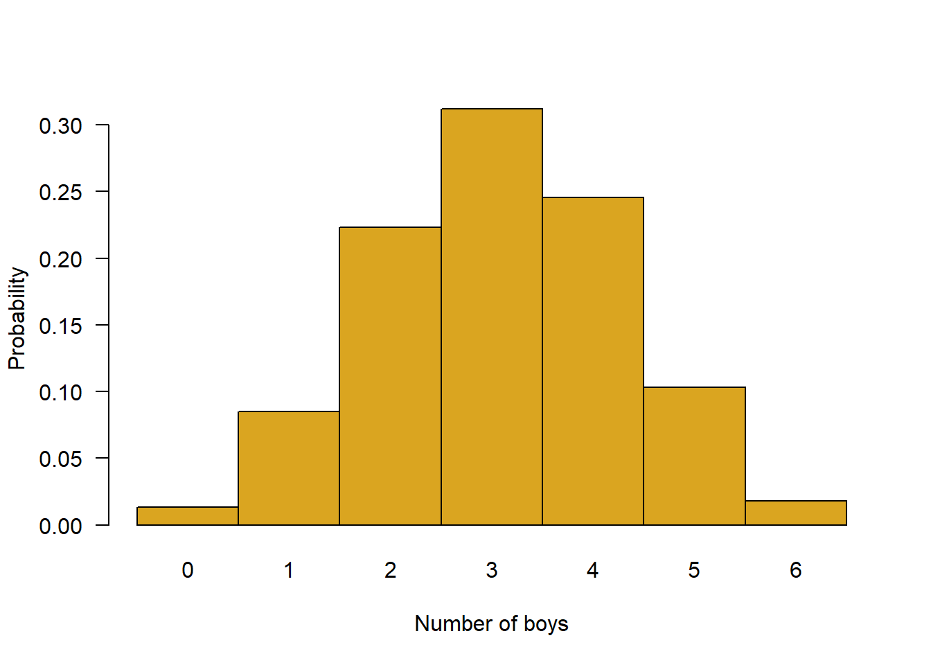
z <- dbinom(0:6,        # number of successes
            size = 6,   # number of trials
            p = 0.512)  # probability of success

# Plot the probability distribution
names(z) <- as.character(0:6) # make the x-axis scale values

barplot(z,                       # data to plot
        space = 0,               # no space between bars
        ylab = "Probability",    # y-axis label
        xlab = "Number of boys", # x-axis label
        col = "goldenrod",       # bar colour
        las = 1)                 # rotate x-axis labels

If mortality is independent of age, then the probability of surviving X years after birth, and then dying in the X + 1st year, will follow a geometric distribution (geom()). X is any integer from 0 to infinity. If the probability of dying in any given year is 0.1, what fraction of individuals are expected to survive 10 years and then die in their 11th year?*

# Calculate the probability
dgeom(10, 0.1)

[1] 0.03486784

Refer to the previous question. If the probability of death in any give year is 0.1, what fraction of individuals die before they reach their 6th birthday?**

# sum the probabilities of dying in years 0 through 5
sum(dgeom(0:5, 0.1))

[1] 0.468559

In an environment where prey are randomly distributed, the search time between discovered prey items will follow an exponential distribution. Imagine an environment in which the mean search time between prey items is 0.5 hours. What is the probability density corresponding to a search time of 2 hours?

# Calculate the probability
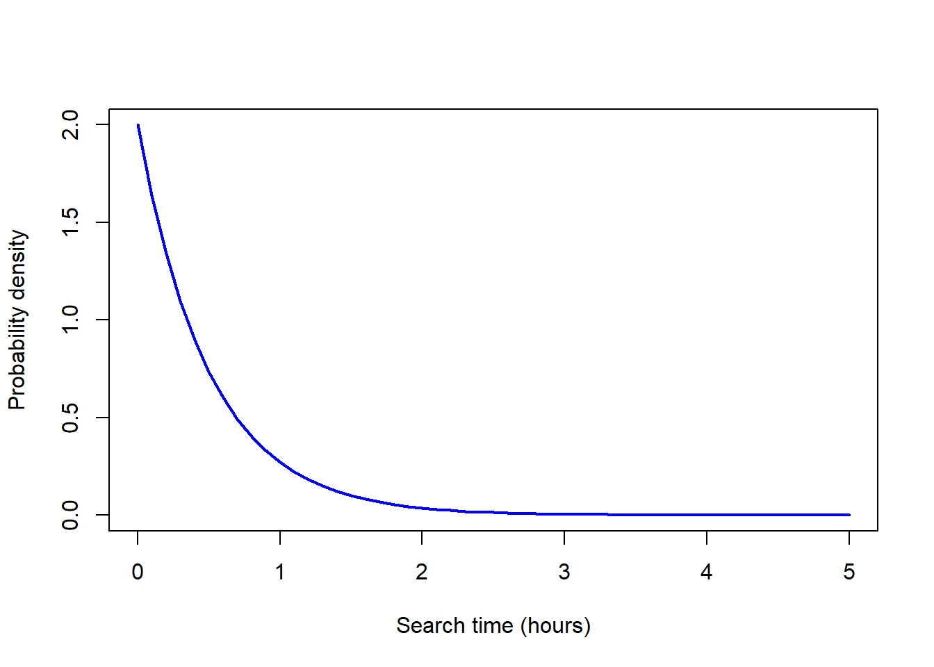
dexp(2, rate = 1/0.5)

[1] 0.03663128

Refer to the previous problem. Create a line plot of the exponential probability curve over most the range of possible values for search time between items (e.g., over the range of values between 0 and 5 hours).

# Make the x-axis scale values
x <- seq(0, 5, by = 0.1)

# Calculate the probability
y <- dexp(x, rate = 1/0.5)

# Plot the probability distribution
plot(y ~ x, type = "l", 
     xlab = "Search time (hours)",
     ylab = "Probability density",
      col = "blue", lwd = 2) # line colour and width

4 Activities

4.1 Left-Handed flowers

Individuals of most plant species are hermaphrodites (with both male and female sexual organs) and are therefore prone to inbreeding. The mud plantain, Heteranthera multiflora (a species of water hyacinth), has a simple mechanism to avoid such “selfing.” The style deflects to the left in some individuals and to the right in others. The anther is on the opposite side. Bees visiting a left-handed plant are dusted with pollen on their right side, which then is deposited on the styles of only right-handed plants visited later.

To investigate the genetics of this variation, Jesson and Barrett (2002) crossed pure strains of left- and right-handed flowers, yielding only right-handed F1 offspring, which were then crossed with one another. Six of the resulting F2 offspring were left-handed, and 21 were right-handed. The expectation under a simple model of inheritance would be that their F2 offspring should consist of left- and right-handed individuals in a 1:3 ratio (i.e., 1/4 of the plants should be left-handed), assuming simple genetic assortment of 2 alleles for 1 locus. You will explore this hypothesis by completing the following tasks:

Generate a vector that includes a range of possible values for the population proportion of left-handed flowers, p, from 0.01 to 0.99 in increments of 0.01.
Given the results above, calculate the log-likelihood of each value for p in the F2 generation.
Create a line plot of the log-likelihood against the range of values for p. What is the resulting curve called? Can you see approximately the value of p corresponding to the highest point of the curve? What is this value called?
To get closer to this value, repeat steps (1) to (3) using a narrower range of values for p surrounding the highest point in the curve and an additional decimal point.
Use your results to determine the maximum likelihood estimate of the proportion of left-handed F2 flowers.
Provide a likelihood-based 95% confidence interval for the population proportion.*
Use the bbmle package to find the maximum likelihood estimate and 95% confidence interval for the proportion of left-handed flowers. How do the results compare with your calculations?
We can compare the fits of two models to these same data, to test the null hypothesis that the proportion of left-handed flowers in the cross is 1/4 (i.e., the proportion predicted by the simplest genetic model for flower handedness). To begin, obtain the log-likelihood corresponding to the maximum likelihood estimate of the proportion of left-handed flowers. This represents the fit of the “full” model to the data. This model estimated one parameter from the data (p, estimated using maximum likelihood).
Now obtain the log-likelihood of the value for p specified by the null hypothesis. This represents the fit of the “reduced” model to the data. This reduced model estimated zero parameters from the data (instead, p was specified by the null hypothesis).
Calculate the G statistic for the log-likelihood ratio test**. To obtain a P-value for the test, calculate the tail probability from the χ2 distribution as follows:

1 - pchisq(G, df)

where df is the degrees of freedom, calculated as the difference between the two models in the number of parameters estimated from the data.

How similar is the result from your log-likelihood ratio test to that from an ordinary χ2 goodness of fit test? Analyse the same data using the chisq.test() command in R and comment on the outcome.

💡 Click here to view a solution

library(tidyverse)
library(bbmle)

# 1. Generate a vector of p values
p_values <- seq(0.01, 0.99, by = 0.01)

# 2. Calculate log-likelihood for each p
log_likelihood <- function(p, n_left, n_right) {
  n <- n_left + n_right
  ll <- n_left * log(p) + n_right * log(1 - p)
  return(ll)
}

n_left <- 6
n_right <- 21
ll_values <- sapply(p_values, log_likelihood, n_left, n_right)

# 3. Create a line plot
plot_data <- tibble(p = p_values, log_likelihood = ll_values)
ggplot(plot_data, aes(x = p, y = log_likelihood)) +
  geom_line() +
  labs(title = "Log-Likelihood Plot", x = "Proportion of Left-Handed Flowers (p)", y = "Log-Likelihood")

# 4. Narrow down the range for p
p_values_fine <- seq(0.05, 0.15, by = 0.001)
ll_values_fine <- sapply(p_values_fine, log_likelihood, n_left, n_right)

# 5. Determine MLE for p
mle_p <- p_values_fine[which.max(ll_values_fine)]

# 6. Likelihood-based 95% CI
# Define the profile likelihood function
profile_likelihood <- function(p) {
  -2 * (log_likelihood(p, n_left, n_right) - log_likelihood(mle_p, n_left, n_right))
}

ci_bounds <- uniroot(profile_likelihood, c(0.094, mle_p))$root
ci_bounds <- c(ci_bounds, uniroot(profile_likelihood, c(mle_p, 0.400))$root)

# 7. Using bbmle package
mle_model <- mle2(minuslogl = function(p) -log_likelihood(p, n_left, n_right), 
                  start = list(p = mle_p), 
                  method = "L-BFGS-B", 
                  lower = 0.01, 
                  upper = 0.99)
summary(mle_model)
confint(mle_model)

# 8. Log-likelihood for MLE
ll_mle <- log_likelihood(mle_p, n_left, n_right)

# 9. Log-likelihood under null hypothesis
p_null <- 0.25
ll_null <- log_likelihood(p_null, n_left, n_right)

# 10. Log-likelihood ratio test
G <- 2 * (ll_mle - ll_null)
p_value <- 1 - pchisq(G, df = 1)

# 11. Chi-square goodness of fit test
chisq.test(c(6, 21), p = c(0.25, 0.75))

4.2 Voyaging voles

The movement or dispersal distance of organisms is often modeled using the geometric distribution, assuming steps are discrete rather than continuous. For example, M. Sandell, J. Agrell, S. Erlinge, and J. Nelson (1991. Oecologia 86: 153-158) measured the distance separating the locations where individual voles, Microtus agrestis, were first trapped and the locations they were caught in a subsequent trapping period, in units of the number of home ranges.

The data for 145 male and female voles are in the file vole.csv. The variable “dispersal” indicates the distance moved (number of home ranges) from the location of first capture. If the geometric model is adequate, then Pr[X = 0 home ranges moved] = p Pr[X = 1 home ranges moved] = (1-p)p Pr[X = 2 home ranges moved] = (1-p)2p and so on. p is the probability of success (capture) at each distance from the location of the first capture. Use this data to complete the following tasks:

Tabulate the number of home ranges moved by voles in this study. Use the data from both sexes combined.
Using the appropriate commands in R, calculate the log-likelihood of each of a range of possible values for p, the parameter of the geometric distribution. Plot the log likelihood against p.
Calculate the maximum-likelihood estimate of p and the likelihood based 95% confidence interval.
Use the appropriate R command and the maximum likelihood estimate of p to calculate the predicted fraction of voles dispersing 0, 1, 2, 3, 4, and 5 home ranges.
Use the result in (3) to calculate the expected number* of voles (out of 145) dispersing 0 - 5 home ranges, assuming a geometric distribution. How does this compare with the observed frequencies?

💡 Click here to view a solution

x <- read.csv("data/vole.csv", 
        stringsAsFactors = FALSE)
        
head(x)

# 1. Tabulate number of home ranges moved
table(x$dispersal)

# 2. MLE of p
p <- seq(0.05, 0.95, by = 0.001)

# Using for loop
# make a vector to store values we will calculate
loglike <- vector()

for(i in 1:length(p)){
    loglike[i] <- sum(dgeom(x$dispersal, prob=p[i], log = TRUE) )
    }

plot(p, loglike, type="l", 
      xlab="p", ylab="log likelihood",
      col = "blue", lwd = 2)

# 3. MLE of p
max(loglike)


phat <- p[loglike == max(loglike)]
z <- p[loglike < max(loglike) - 1.92]
c( max(z[z < 0.858]), min(z[z > 0.858]) )

# 4. Expected numbers 
frac <- dgeom(0:5, prob=phat)
round(frac,4)

expected <- frac * nrow(x)

round(expected, 2)

# Use the maximum likelihood estimate of p to calculate the 
# predicted fraction of voles dispersing 0, 1, 2, 3, 4, and 5 home ranges.
frac <- dgeom(0:5, prob=phat)
round(frac,4)

# Expected distances moved
dist <- nrow(x) * frac
round(dist, 2)

# Compare with observed:
table(x$dispersal)

4.3 Bees

The life span of individuals in a population are often approximated by an exponential distribution. To estimate the mortality rate of foraging honey bees, scientists have recorded the entire foraging life span of 33 individual worker bees in a local bee population in a natural setting. The 33 life spans (in hours) are in the file bees.csv. Use this data to complete the following tasks:

Plot the frequency distribution of lifespans of the 33 bees. Choose the option to display probability density instead of raw frequency. Does the distribution of lifespans resemble an exponential distribution (make sure to try different bin widths of the histogram)?
Use the exponential approximation and maximum likelihood to estimate the hourly mortality rate of bees.
Using the maximum likelihood estimate, calculate the probability density for the exponential distribution across a range of values for lifespan. Draw this relationship between probability and lifespan on top of the frequency distribution you plotted in (1). Comment on the fit between the data and the exponential distribution you fitted. Is the exponential distribution a good fit to these data?
Assume (for the purposes of this exercise) that an exponential probability model is reasonable. Calculate the likelihood-based 95% confidence interval for the mortality rate.**
Calculate the maximum likelihood estimate for the mean lifespan, with approximate 95% likelihood based confidence interval.

💡 Click here to view a solution

bees <- read.csv("data/bees.csv", 
          stringsAsFactors = FALSE)
          
head(bees)

# 1. Plot histogram

hist(bees$hours, right = FALSE, col = "goldenrod", prob = TRUE, 
      ylim = c(0,0.035), las = 1, breaks = 15)

# 2. MLE of rate (in per hour units)
rate <- seq(.001, .1, by=.001)

# Using for loop
loglike <- vector()

for(i in 1:length(rate)){
    loglike[i] <- sum(dexp(bees$hours, rate = rate[i], log = TRUE))
    }

plot(rate, loglike, type="l",
    col = "blue", lwd = 2)

max(loglike)

mlrate <- rate[loglike==max(loglike)] # per hour
mlrate

# 3. Exponential might not be a great fit
hist(bees$hours, right = FALSE, col = "goldenrod", prob = TRUE, 
      ylim = c(0,0.035), las = 1, breaks = 15)

x <- bees$hours[order(bees$hours)]
y <- dexp(x, rate = 0.036)
lines(x, y, lwd=2)

# 4. 95% confidence interval
z <- rate[loglike < max(loglike) - 1.92]
c( max(z[z < mlrate]), min(z[z > mlrate]) )

# 5. Mean lifespan
1/mlrate

1/c( max(z[z < mlrate]), min(z[z > mlrate]) )

1 Objectives

2 Start a Script

3 Introduction

3.1 Maximum likelihood estimate

3.2 Log-likelihood ratio test

3.3 Basic R commands

4 Activities

4.1 Left-Handed flowers

4.2 Voyaging voles

4.3 Bees

3.3 Basic `R` commands