1 Objectives

Calculate a correlation coefficient and the coefficient of determination;
Test hypotheses about correlation;
Use the non-parametric Spearman’s correlation.

2 Start a Script

For this lab or project, begin by:

Starting a new R script
Create a good header section and table of contents
Save the script file with an informative name
set your working directory

Aim to make the script a future reference for doing things in R!

3 Introduction

Most of you will have heard the maxim “correlation does not imply causation”. Just because two variables have a statistical relationship with each other does not mean that one is responsible for the other. For instance, ice cream sales and forest fires are correlated because both occur more often in the summer heat. But there is no causation; you don’t light a patch of the Montana brush on fire when you buy a pint of Haagan-Dazs.

A correlation is a statistical measure of an association between two variables. An association is any relationship between the variables that makes them dependent in some way: knowing the value of one variable gives you information about the possible values of the other.

The terms ‘association’ and ‘correlation’ are often used interchangeably but strictly speaking correlation has a narrower definition. A correlation quantifies, via a measure called a correlation coefficient, the degree to which an association tends to a certain pattern. For example, the correlation coefficient studied below—Pearson’s correlation coefficient—measures the degree to which two variables tend toward a straight line relationship.

4 Correlation

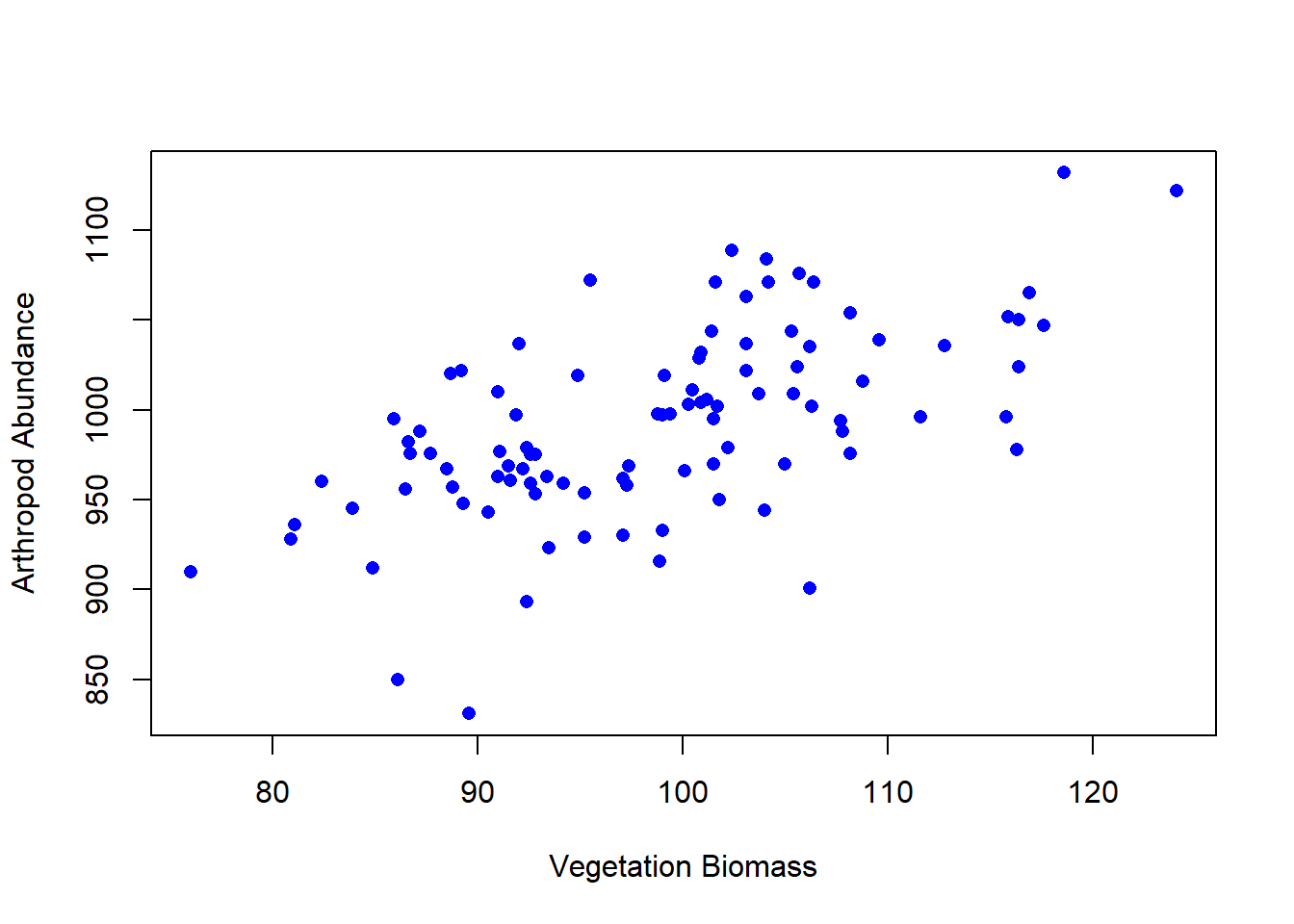
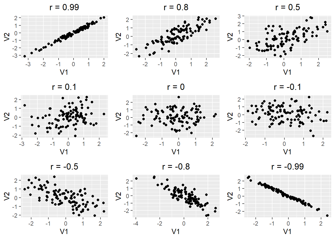
The question of correlation is simply whether there is a demonstrable association between two numeric variables. For example, we might wonder this for two numeric variables, such as a measure of vegetation biomass and a measure of insect abundance. Digging a little deeper, we are interested in seeing and quantifying whether and how the variables may “co-vary” (i.e, exhibit significant covariance). This covariance may be quantified as being either positive or negative and may vary in strength from zero, to perfect positive or negative correlation (+1, or -1). We traditionally visualise correlation with a scatterplot (plot() in R). For example, we can see in the figure below that the two variables tend to increase with each other positively, suggesting a positive correlation.

There are different methods for quantifying correlation but these all share a number of properties:

If there is no relationship between the variables the correlation coefficient will be zero. The closer to 0 the value, the weaker the relationship. A perfect correlation will be either -1 or +1, depending on the direction;
The value of a correlation coefficient indicates the direction and strength of the association but says nothing about the steepness of the relationship. A correlation coefficient is just a number, so it can’t tell us exactly how one variable depends on the other;
Correlation coefficients do not describe ‘directional’ or ‘casual’ relationships—i.e. we can’t use correlations to make predictions about one variable based on knowledge of another or make statements about the effect of one variable on the other;
A correlation coefficient doesn’t tell us whether an association is likely to be ‘real’ or not. We have to use a statistical significance test to evaluate whether a correlation may be different from zero. Like any statistical test, this requires certain assumptions about the variables to be met.

Warning: package 'gridExtra' was built under R version 4.3.2

5 Pearson’s Correlation Coefficient

What do we need to know about Pearson’s product-moment correlation? Let’s start with the naming conventions. People often use “Pearson’s correlation coefficient” or “Pearson’s correlation” as a convenient shorthand because writing “Pearson’s product-moment correlation coefficient” all the time soon becomes tedious. If we want to be really concise we use the standard mathematical symbol to denote Pearson’s correlation coefficient—lower case ‘r’.

The one thing we absolutely have to know about Pearson’s correlation coefficient is that it is a measure of linear association between numeric variables. This means Pearson’s correlation is appropriate when numeric variables follow a ‘straight-line’ relationship. That doesn’t mean they have to be perfectly related, by the way. It simply means there shouldn’t be any ‘curviness’ to their pattern of association5.

Finally, calculating Pearson’s correlation coefficient serves to estimate the strength of an association. An estimate can’t tell us whether that association is likely to be ‘real’ or not. We need a statistical test to tackle that question. There is a standard parametric test associated with Pearson’s correlation coefficient. Unfortunately, this does not have its own name. We will call it “Pearson’s correlation coefficient” to distinguish the test from the actual correlation coefficient. Just keep in mind these are not ‘official’ names.

Pearson’s correlation coefficient is calculated by dividing the covariance of the two variables by the product of their standard deviations. The formula for calculating r is as follows:

\[r = \frac{\sum_{i=1}^{n}(x_i - \bar{x})(y_i - \bar{y})}{\sqrt{\sum_{i=1}^{n}(x_i - \bar{x})^2}\sqrt{\sum_{i=1}^{n}(y_i - \bar{y})^2}}\]

where:

\(x_i\) is the \(i^{th}\) value of the x-variable
\(y_i\) is the \(i^{th}\) value of the y-variable
\(\bar{x}\) is the mean of the x-variable
\(\bar{y}\) is the mean of the y-variable

The formula for calculating r is complex and tedious to calculate by hand. Fortunately, R has a built-in function to calculate r called cor(). The cor() function takes two arguments, the x-variable and the y-variable, and returns the correlation coefficient. For example, to calculate the correlation coefficient for the vegetation biomass and arthropod abundance data, we type:

cor(veg, arth, method = "pearson")

[1] 0.6056694

The correlation coefficient is 0.605, which indicates a moderate positive correlation between the two variables. We can also calculate the correlation coefficient for the vegetation biomass and arthropod abundance data using the cor.test() function. The cor.test() function takes the same arguments as the cor() function, but it also calculates a p-value to test the null hypothesis that the correlation coefficient is equal to zero. For example, to calculate the correlation coefficient and p-value for the vegetation biomass and arthropod abundance data, we type:

cor.test(~ veg + arth, method = "pearson")


    Pearson's product-moment correlation

data:  veg and arth
t = 7.4966, df = 97, p-value = 3.101e-11
alternative hypothesis: true correlation is not equal to 0
95 percent confidence interval:
 0.4637006 0.7173146
sample estimates:
      cor 
0.6056694

When using Pearson’s method we report the value of the correlation coefficient, the sample size, and the p-value6. Here’s how to report the results of this analysis: there is a moderate positive correlation between vegetation biomass and arthropod abundance (r = 0.605, n = 100, p < 0.001).

6 Spearman’s Rank Correlation Coefficient

An alternative to the Pearson correlation (the traditional correlation, assuming the variables in question are Gaussian), is the Spearman rank correlation, which can be used when the assumptions for the Pearson correlation are not met. These assumptions are:

Linearity - the relationship between the two variables is linear, meaning the best-fit line through the data points is a straight line. Pearson’s correlation may not be appropriate or may give misleading results if the relationship is not linear;
Bivariate normality - both variables should be normally distributed. More specifically, the joint distribution of the two variables should be bivariate normal. This assumption means that for any fixed value of one variable, the distribution of the other variable should be normal, and vice versa;
Homoscedasticity - this means that the variance of one variable is constant at all levels of the other variable. In other words, the data should form a roughly oval-shaped scatter plot;
Independence of observations - each pair of observations (x, y) is independent of other pairs. This assumption is crucial for the validity of the statistical inferences made using Pearson’s correlation;
Absence of outliers - Pearson’s correlation is sensitive to outliers. Outliers can have a disproportionate effect on the correlation coefficient, either inflating or deflating its value.

The Spearman rank correlation coefficient is commonly denoted by rho. It is calculated by dividing the covariance of the ranks of the two variables by the product of their standard deviations. The formula for calculating r_s is as follows:

\[rho = \frac{\sum_{i=1}^{n}(x_i - \bar{x})(y_i - \bar{y})}{\sqrt{\sum_{i=1}^{n}(x_i - \bar{x})^2}\sqrt{\sum_{i=1}^{n}(y_i - \bar{y})^2}}\]

where:

\(x_i\) is the \(i^{th}\) rank of the x-variable
\(y_i\) is the \(i^{th}\) rank of the y-variable
\(\bar{x}\) is the mean of the ranks of the x-variable
\(\bar{y}\) is the mean of the ranks of the y-variable

The formula for calculating r_s is complex and tedious to calculate by hand. Fortunately, R has a built-in function to calculate r_s called cor(). The cor() function takes two arguments, the x-variable and the y-variable, and returns the correlation coefficient. For example, to calculate the correlation coefficient for some data on soil pH and crop yield we run:

set.seed(42) # For reproducibility

# Number of observations
n <- 100

# Generating data
# Soil pH - Uniformly distributed between 3.5 and 9
soil_ph <- runif(n, min = 3.5, max = 9)

# Crop Yield - Non-linear relationship with soil pH
crop_yield <- 100 - ((soil_ph - 6)^2 + rnorm(n, sd = 5)) * 10

# Create a data frame
agri_data <- data.frame(Soil_pH = soil_ph, Crop_Yield = crop_yield)

# Perform Spearman's correlation test
cor.test(agri_data$Soil_pH, agri_data$Crop_Yield, method = "spearman")


    Spearman's rank correlation rho

data:  agri_data$Soil_pH and agri_data$Crop_Yield
S = 217970, p-value = 0.001909
alternative hypothesis: true rho is not equal to 0
sample estimates:
       rho 
-0.3079508

The correlation coefficient is -0.308 and the p-value is < 0.001, which indicates a negative correlation between the two variables. The p-value is less than 0.05, which indicates that the correlation coefficient is significantly different from zero. Therefore, we can reject the null hypothesis that the correlation coefficient is equal to zero and conclude that there is a significant correlation between the two variables.

7 Activities

7.1 Graphical correlation

Load the waders data from the MASS package and read the help page. Use the pairs function on the data and make a statement about the overall degree of intercorrelation between variables based on the graphical output.

💡 Click here to view a solution

7.2 Correlation

Think about the variables and data themselves in waders. Do you expect the data to be Gaussian? Formulate hypothesis statements for correlations amongst the first 3 columns of bird species in the data set. Show the code to make three good graphs (i.e., one for each pairwise comparison for the first three columns), and perform the three correlation tests. What do you conclude?

💡 Click here to view a solution

7.3 Validation

Validate the test performed in question 2. Which form of correlation was performed, and why. Show the code for any diagnostic tests performed, and any adjustment to the analysis required. Formally report the results of your validated results.

💡 Click here to view a solution