# Graphing arguments in plot(), boxplot(), hist() etc.
# main = "Eureka!" # add a title above the graph
# pch = 16 # set plot symbol to a filled circle
# color = "red" # set the item color
# xlim = c(-10,10) # set limits of the x-axis (horizontal axis)
# ylim = c(0,100) # set limits of the y-axis (vertical axis)
# lty = 2 # set line type to dashed
# las = 2 # rotate axis labels to be perpendicular to axis
# cex = 1.5 # magnify the plotting symbols 1.5-fold
# cex.lab = 1.5 # magnify the axis labels 1.5-fold
# cex.axis = 1.3 # magnify the axis annotation 1.3-fold
# xlab = "Body size" # label for the x-axis
# ylab = "Frequency" # label for the y-axis1 Learning Objectives
- Review some basic graphical formats and when they are useful;
- Learn key tools for creating graphs in
R; - Make some basic graphs in
R.
2 Introduction
Data visualisation is a critical skill for the modern scientist. An ability to create insightful, engaging data graphics is invaluable for research, collaborations, and science communication. Good data visualisation requires appreciation and careful consideration of the technical aspects of data presentation. But it also involves a creative element. Authorial choices are made about the “story” we want to tell, and design decisions are driven by the need to convey that story most effectively to our audience. Software systems use default settings for most graphical elements. However, each visualisation has its own story to tell, and so we must actively consider and choose settings for the visualisation under construction. In this lab, we will learn various basic plotting coding techniques using both base R and ggplot2.
3 Base R vs ggplot2
3.1 Context
R has a rich ecosystem for data visualization, with the main frameworks being base R graphics and ggplot2. Base R graphics are the foundational plotting system, great for quick and simple visualisations. It is built directly into R, so no extra package installations are required. However, it can become complex for more intricate plots. ggplot2 is part of the tidyverse and allows for more complex and aesthetically pleasing graphics. This package uses a layered, declarative approach based on the grammar of graphics, making it easier to produce and modify complex plots. It is also highly extensible and has a strong community support. You should choose the tool that fits your specific needs, but mastering one well is often more beneficial than a superficial understanding of many. This lab will focus on base R and ggplot2. Understanding the R data visualisation ecosystem will not only allow you to create compelling visualisations but also make your research more impactful. There is, however, some controversy as to whether you should use ggplot2 - see Leek (2016) and Robinson (2016).
3.2 Base R
Many of the basic plotting commands in base R will accept the same arguments to control axis limits, labeling, and other options. If you are not sure whether a given option works in your case, try it. The worst that could happen is you get an error message, or R simply ignores you.
For details and the full list of plotting options in base R, run:
# Graphical parameters
?par

# Basic plot decorations
?plot.default
3.3 ggplot2
ggplot2is a system for declaratively creating graphics, based on The Grammar of Graphics. You provide the data, tellggplot2how to map variables to aesthetics, what graphical primitives to use, and it takes care of the details.
Building a graph using the ggplot() function involves the combination of components, or “layers”, including data, that you build up and connect using the + symbol. You use a few kinds of commands including “aesthetics” (using aes()) to map variables to visuals, and different “geoms” functions to create different kinds of plots. A ggplot is built up from a few basic elements:
- Data: The raw data that you want to plot.
- Geometries
geom_: The geometric shapes that will represent the data. - Aesthetics
aes(): Aesthetics of the geometric and statistical objects, such as position, color, size, shape, and transparency - Scales
scale_: Maps between the data and the aesthetic dimensions, such as data range to plot width or factor values to colours. - Statistical transformations
stat_: Statistical summaries of the data, such as quantiles, fitted curves, and sums. - Coordinate system
coord_: The transformation used for mapping data coordinates into the plane of the data rectangle. - Facets
facet_: The arrangement of the data into a grid of plots. - Visual themes
theme(): The overall visual defaults of a plot, such as background, grids, axes, default typeface, sizes and colors.
💡 The number of elements may vary depending on how you group them and whom you ask.
The syntax of ggplot2 is different from base R. In accordance with the basic elements, a default ggplot needs three things that you have to specify: the data, aesthetics, and a geometry. We always start to define a plotting object by calling ggplot(data = df) which just tells ggplot2 that we are going to work with that data. In most cases, you might want to plot two variables—one on the x and one on the y axis. These are positional aesthetics and thus we add aes(x = var1, y = var2) to the ggplot() call (yes, the aes() stands for aesthetics). However, there are also cases where one has to specify one or even three or more variables.
💡 We specify the data outsideaes() and add the variables that ggplot maps the aesthetics to insideaes().
4 Lab Environment
4.1 Start a Script
For this lab or project, begin by:
- Starting a new
Rscript - Create a good header section and table of contents
- Save the script file with an informative name
- set your working directory
Aim to make the script a future reference for doing things in R!
4.2 Packages
We need to install and load palmerpenguins to access the data and tidyverse to access the ggplot2 package:
# Check whether a package is installed and install if not
if(!require("palmerpenguins")) install.packages("palmerpenguins")
Loading required package: palmerpenguinsWarning: package 'palmerpenguins' was built under R version 4.3.2if(!require("tidyverse")) install.packages("tidyverse")Loading required package: tidyverse── Attaching core tidyverse packages ──────────────────────── tidyverse 2.0.0 ──
✔ dplyr 1.1.3 ✔ readr 2.1.4
✔ forcats 1.0.0 ✔ stringr 1.5.0
✔ ggplot2 3.4.4 ✔ tibble 3.2.1
✔ lubridate 1.9.3 ✔ tidyr 1.3.0
✔ purrr 1.0.2
── Conflicts ────────────────────────────────────────── tidyverse_conflicts() ──
✖ dplyr::filter() masks stats::filter()
✖ dplyr::lag() masks stats::lag()
ℹ Use the conflicted package (<http://conflicted.r-lib.org/>) to force all conflicts to become errors# Load packages
library(palmerpenguins, quietly = TRUE)
library(tidyverse, quietly = TRUE)4.3 Data
You will be using the Palmer Penguins dataset to produce your own EDA graphs. This dataset was collected and made available by Dr Kristen Gorman and the Palmer Station, Antarctica LTER, a member of the Long Term Ecological Research Network.
There are two datasets within the palmerpenguins package. The first is called penguins and is a simplified version of the raw data while the second is called penguins_raw and contains all the variables and original names as downloaded. You are going to use the first penguins data set as it is already in a tidy format.
Let’s take a brief look at the dataset to see what you’re working with. First we need to load the data:
# Load the data set
data(penguins)

# View first 5 rows of data
head(penguins, n = 5)
# A tibble: 5 × 8
species island bill_length_mm bill_depth_mm flipper_length_mm body_mass_g
<fct> <fct> <dbl> <dbl> <int> <int>
1 Adelie Torgersen 39.1 18.7 181 3750
2 Adelie Torgersen 39.5 17.4 186 3800
3 Adelie Torgersen 40.3 18 195 3250
4 Adelie Torgersen NA NA NA NA
5 Adelie Torgersen 36.7 19.3 193 3450
# ℹ 2 more variables: sex <fct>, year <int>Now we can view a summary using the summary() function:
# Display data set summary
summary(penguins)
species island bill_length_mm bill_depth_mm
Adelie :152 Biscoe :168 Min. :32.10 Min. :13.10
Chinstrap: 68 Dream :124 1st Qu.:39.23 1st Qu.:15.60
Gentoo :124 Torgersen: 52 Median :44.45 Median :17.30
Mean :43.92 Mean :17.15
3rd Qu.:48.50 3rd Qu.:18.70
Max. :59.60 Max. :21.50
NA's :2 NA's :2
flipper_length_mm body_mass_g sex year
Min. :172.0 Min. :2700 female:165 Min. :2007
1st Qu.:190.0 1st Qu.:3550 male :168 1st Qu.:2007
Median :197.0 Median :4050 NA's : 11 Median :2008
Mean :200.9 Mean :4202 Mean :2008
3rd Qu.:213.0 3rd Qu.:4750 3rd Qu.:2009
Max. :231.0 Max. :6300 Max. :2009
NA's :2 NA's :2 Okay, so it looks as if the data set contains data for 344 penguins and there are eight variables. There are three different species of penguins in this data set, collected from three islands in the Palmer Archipelago, Antarctica over two years (2007-2009). For each penguin studied we have a range of measurements, including bill length and depth as well as flipper length and body mass. There are some NA values, which might cause us some issues, so let’s remove those:
penguins <- na.omit(penguins)

# Display data set summary
summary(penguins)
species island bill_length_mm bill_depth_mm
Adelie :146 Biscoe :163 Min. :32.10 Min. :13.10
Chinstrap: 68 Dream :123 1st Qu.:39.50 1st Qu.:15.60
Gentoo :119 Torgersen: 47 Median :44.50 Median :17.30
Mean :43.99 Mean :17.16
3rd Qu.:48.60 3rd Qu.:18.70
Max. :59.60 Max. :21.50
flipper_length_mm body_mass_g sex year
Min. :172 Min. :2700 female:165 Min. :2007
1st Qu.:190 1st Qu.:3550 male :168 1st Qu.:2007
Median :197 Median :4050 Median :2008
Mean :201 Mean :4207 Mean :2008
3rd Qu.:213 3rd Qu.:4775 3rd Qu.:2009
Max. :231 Max. :6300 Max. :2009 4.4 Data Documentation
It is important to document the data you are using in your analysis. This is especially important if you are using data from a third party source. Familiarise yourself with the Palmer Penguins data by reading the package documentation Link.
5 Basic Graphs
5.1 Histograms
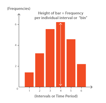
A histogram is a graphical representation of the distribution of a data set. It is an estimate of the probability distribution of a continuous variable. To construct a histogram, the first step is to “bin” the range of values (that is, divide the entire range of values into a series of intervals) and then count how many values fall into each interval. These counts are then represented as bars. Their uses include:
- Distribution Analysis: Histograms are commonly used to visually assess how the data points are distributed with respect to frequency. They can help identify skewness, outliers, or anomalies in the data.
- Identify Patterns: By looking at the shape of the histogram, you can gain insights into the underlying distribution model of the data - whether it’s gaussian, exponential, bimodal, etc.
- Data Segmentation: You can use histograms to segment data into different categories for further analysis. For instance, a histogram could help you identify age groups most affected by a particular disease in epidemiological studies.
- Quality Control: In manufacturing and business processes, histograms can help in identifying the most frequent occurrences of a particular variable, aiding in quality control and decision-making.
- Comparison: Multiple histograms can be plotted together to compare different data sets or different subsets of the same data set.
5.1.1 Histograms in base R
Let’s start by creating a histogram of the flipper length of the penguins. We can use the hist() function to do this:
# Create histogram of flipper length
hist(penguins$flipper_length_mm) # Specify data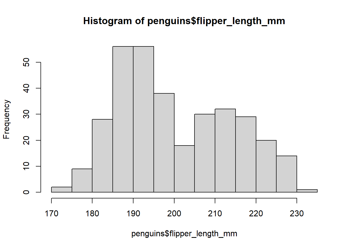
The hist() function has a number of arguments that you can use to customise the histogram. For example, you can change the number of bins using the breaks argument:
# Create histogram of flipper length
hist(penguins$flipper_length_mm, breaks = 5) # Specify data and change number of bins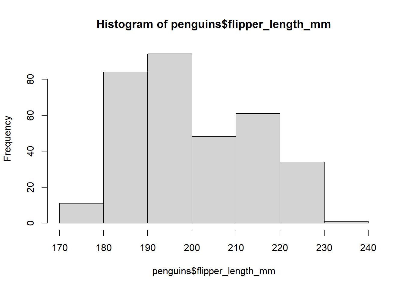
5.1.2 Histograms in ggplot2
Now let’s create the same histogram using ggplot2. We start by specifying the data and the aesthetic mappings:
# Create histogram of flipper length
ggplot(data = penguins, aes(x = flipper_length_mm)) # Specify data and aesthetic mappings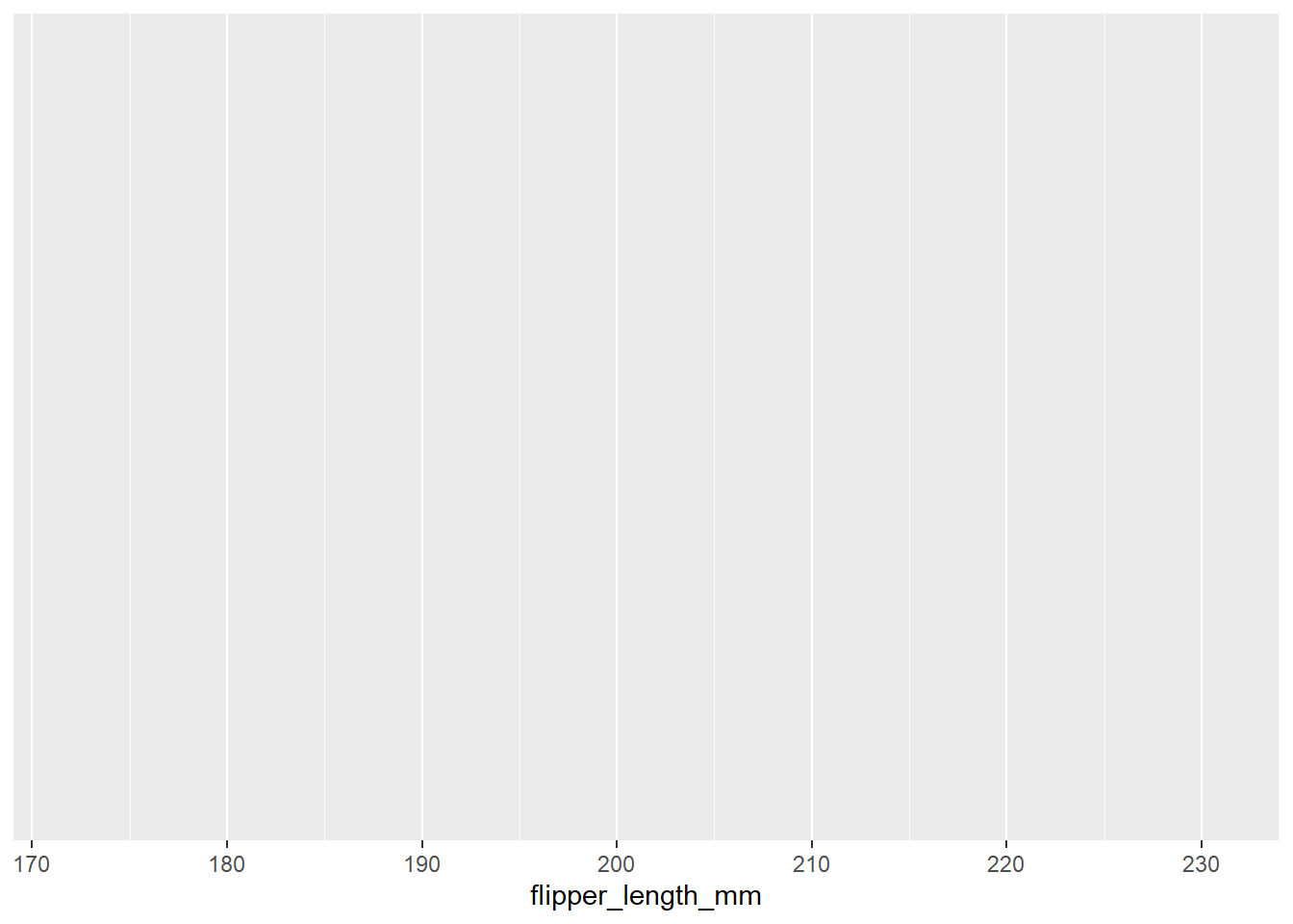
You will see that this produces a blank plot. This is because we have not specified the type of plot we want to create. We can do this using the geom_histogram() function:
# Create histogram of flipper length
ggplot(data = penguins, aes(x = flipper_length_mm)) + # Specify data and aesthetic mappings
  geom_histogram()                                    # Add histogram layer
`stat_bin()` using `bins = 30`. Pick better value with `binwidth`.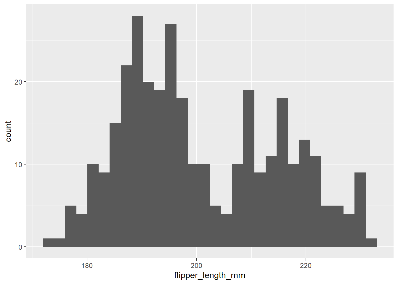
5.1.3 Density Plots
Sometimes, histograms may not be the best approach to visualising distributions! An alternative is the density plot, which visualises the distribution of data over a continuous interval or time period. This chart is a variation of a Histogram that uses kernel smoothing to plot values, allowing for smoother distributions by smoothing out the noise. The peaks of a Density Plot help display where values are concentrated over the interval.

# Plotting a density plot for bill length using ggplot2
ggplot(data = penguins, aes(x = bill_length_mm)) + # Specify data and aesthetic mappings
  geom_density(fill = "darkblue") +                # Change colour
  labs(title = "Density plot of bill length",      # Add title
       x = "Bill length (mm)")                     # Add x-axis label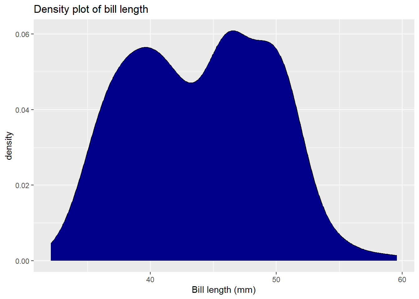
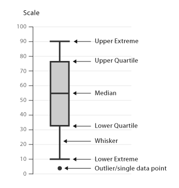
5.2 Boxplots
A boxplot is a graphical representation that provides a five-number summary of a data set: the minimum, first quartile (Q1), median, third quartile (Q3), and maximum. The “box” in the plot represents the interquartile range (IQR), which is the range between Q1 and Q3, and it contains the middle 50% of the data points while “whiskers” extend from the box to show the data spread. Points outside the whiskers are often considered outliers. Their uses include:
- Data Summary: Boxplots provide a quick way to visualize the central tendency and spread of a dataset, making them useful for preliminary data analysis.
- Outlier Detection: One of the most common uses of boxplots is the identification of outliers, which are displayed as individual points beyond the whiskers.
- Comparison: When you have multiple categories of data, boxplots can be used side-by-side to easily compare distributions and identify patterns or discrepancies.
- Assumption Checking: In statistical analysis, boxplots are useful for checking assumptions related to the distribution of the data, homogeneity of variances, among others.
- Skewness and Symmetry: The shape and positioning of the box and whiskers can provide insights into the skewness of the data. A symmetric distribution will have a box and whiskers of roughly equal size.
5.2.1 Boxplots in base R
Let’s start by creating a boxplot of the flipper length of the penguins. We can use the boxplot() function to do this:
# Create boxplot of flipper length
boxplot(penguins$flipper_length_mm) # Specify data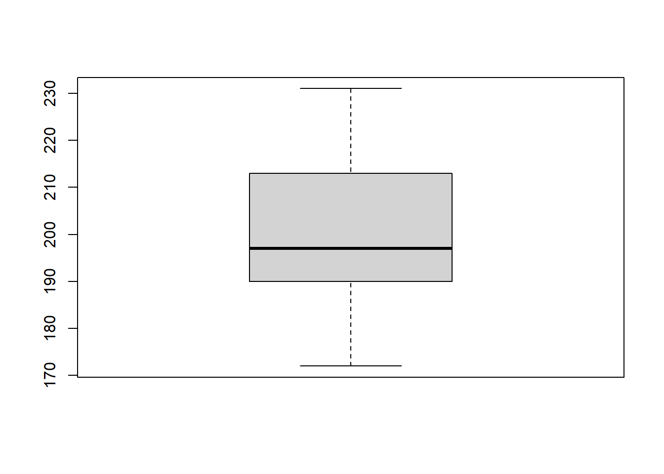
The boxplot() function has a number of arguments that you can use to customise the boxplot. For example, you can change the orientation of the boxplot using the horizontal argument:
5.2.2 Boxplots in ggplot2
Now let’s create the same boxplot using ggplot2. We start by specifying the data and the aesthetic mappings:
# Create boxplot of flipper length
ggplot(data = penguins, aes(x = species, y = flipper_length_mm)) # Specify data and aesthetic mappings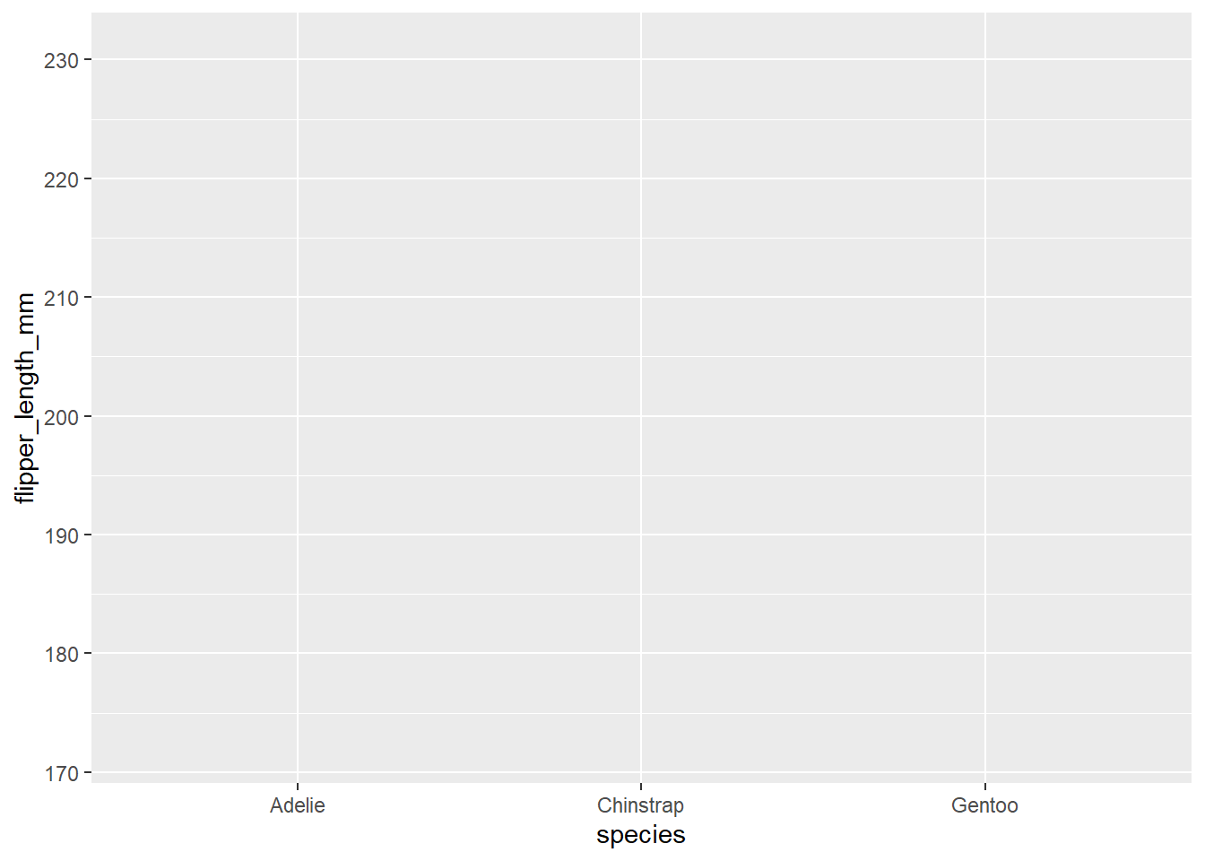
You will see that this produces a blank plot. This is because we have not specified the type of plot we want to create. We can do this using the geom_boxplot() function:
# Create boxplot of flipper length
ggplot(data = penguins, aes(x = species, y = flipper_length_mm)) + # Specify data and aesthetic mappings
  geom_boxplot()                                                   # Add boxplot layer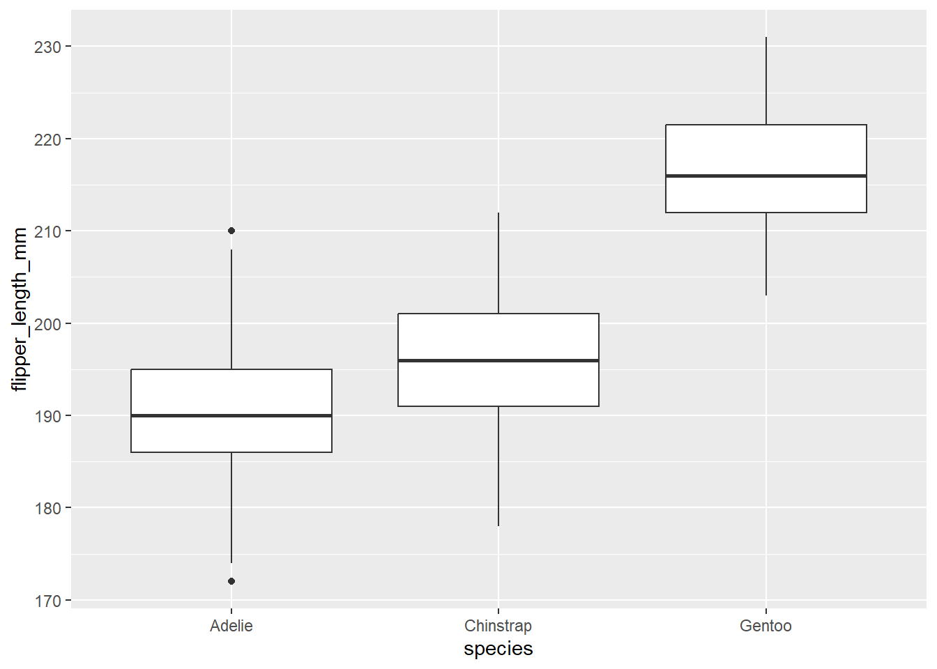
This produces a ggplot2 plot that closely resembles the base R plot. We may also want to overlay the individual data points for a better understanding of the data:
# Create boxplot of flipper length
ggplot(data = penguins, aes(x = species, y = flipper_length_mm)) + # Specify data and aesthetic mappings
  geom_boxplot(data = penguins, aes(fill = species)) +             # Add boxplot layer and change colour by species
  geom_point(data = penguins) +                                    # Add points layer
  labs(title = "Boxplot of flipper length",                        # Add title
       x = "Species",                                              # Add x-axis label
       y = "Flipper length (mm)")                                  # Add y-axis label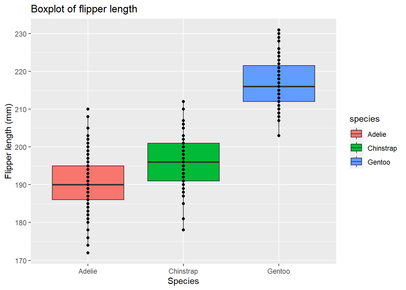
These points are quite clustered, so let’s change their opacity and add a jitter to spread them out:
# Create boxplot of flipper length
ggplot(data = penguins, aes(x = species, y = flipper_length_mm)) + # Specify data and aesthetic mappings
  geom_boxplot(data = penguins, aes(fill = species)) +             # Add boxplot layer and change colour by species
  geom_point(data = penguins,                                      # Add points layer
             alpha = 0.5,                                          # Change opacity
             position = position_jitter(width = 0.1)) +            # Add jitter
  labs(title = "Boxplot of flipper length",                        # Add title
       x = "Species",                                              # Add x-axis label
       y = "Flipper length (mm)")                                  # Add y-axis label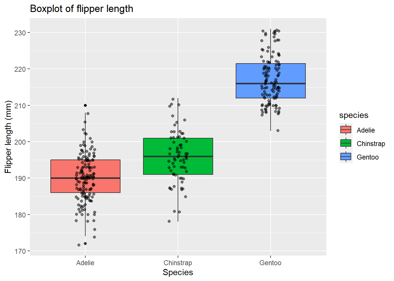
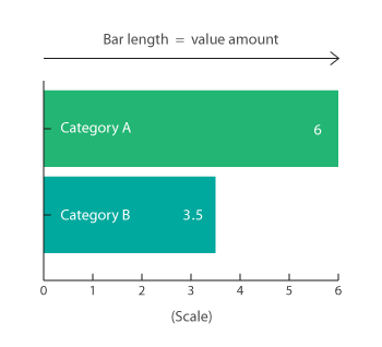
5.3 Barplots
Barplots are used to display the distribution of categorical data. They are similar to histograms, but they are used for discrete data, whereas histograms are used for continuous data. Barplots are also used to compare the values of a variable at a given point in time. Their uses include:
- Data Comparison: One of the primary uses of bar plots is to compare data across categories. For example, you might use a bar plot to compare the sales of different products in a store.
- Frequency Distribution: Bar plots can display the frequency of different categories in a data set, making them useful for understanding the data distribution.
- Data Summarisation: They are excellent for summarizing data from surveys or experiments into easily interpretable visual forms.
- Trend Identification: While not as nuanced as line graphs for displaying trends, bar plots can still effectively show general trends over time when the time intervals are discrete.
- Part-to-Whole Relationships: Stacked bar plots can show how individual categories contribute to an overall total, helping to understand part-to-whole relationships.
5.3.1 Barplots in base R
Let’s start by creating a barplot of the species of penguins in the dataset. We can use the barplot() function to do this:
# Create barplot of species
barplot(table(penguins$species)) # Specify data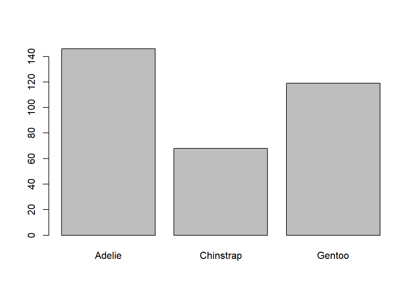
5.3.2 Barplots in ggplot2
Now let’s create the same barplot using ggplot2. We start by specifying the data and the aesthetic mappings:
# Create barplot of species
ggplot(data = penguins, aes(x = species)) # Specify data and aesthetic mappings
You will see that this produces a blank plot. This is because we have not specified the type of plot we want to create. We can do this using the geom_bar() function:
# Create barplot of species
ggplot(data = penguins, aes(x = species)) + # Specify data and aesthetic mappings
  geom_bar()                                # Add bar plot layer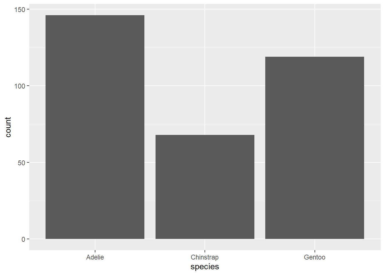
We can see that this produces the same barplot as the base R version.
5.3.3 Grouped barplots
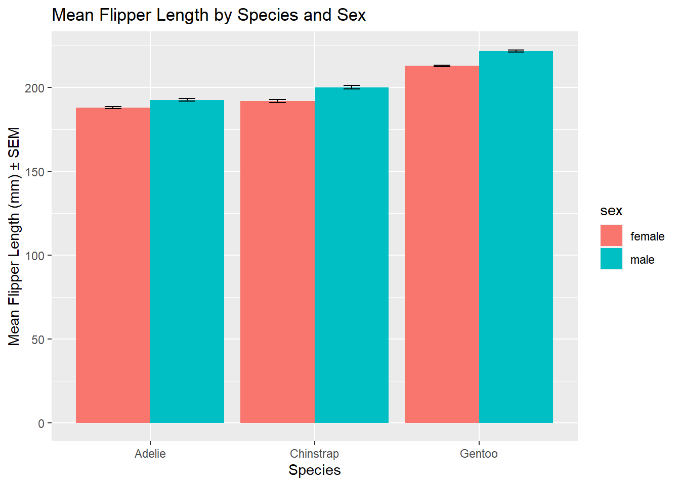
As scientists it is not often that we want to create such simple barplots - we might want to compare two or more groups along with some measure of variation. For this we need to use a grouped barplot. Let’s say we are interested in visualising the mean flipper length of penguins, grouped by species and sex, along with the standard error of the mean for each group. We can do this using the geom_bar() function:
# Calculate the mean and standard error of the mean (SEM) for flipper length, grouped by species and sex
grouped_data <- penguins %>%                               # Specify data
  group_by(species, sex) %>%                               # Group data
  summarise(mean_flipper_length = mean(flipper_length_mm), # Calculate mean
            sem = sd(flipper_length_mm) / sqrt(n()),       # Calculate SEM = standard deviation / sqrt(n)
            .groups = 'drop')                              # Drop groups
In the above code we have used the pipe (%>%) operator to pipe the data into the group_by() function. This is a useful way of chaining together multiple functions. We have also used the summarise() function to calculate the mean and standard error of the mean (SEM) for each group. We have then used the ggplot() function to create the plot, specifying the data and aesthetic mappings:
# Create the ggplot
ggplot(grouped_data, aes(x = species, y = mean_flipper_length, fill = sex)) +             # Specify data and aesthetic mappings
  geom_bar(stat = "identity", position = "dodge") +                                       # Add bar plot layer
  geom_errorbar(aes(ymin = mean_flipper_length - sem, ymax = mean_flipper_length + sem),  # Add error bars
                width = 0.2, position = position_dodge(0.9)) +                            # Specify width and position of error bars
  labs(
    title = "Mean Flipper Length by Species and Sex",                                     # Add title
    x = "Species",                                                                        # Add x-axis label
    y = "Mean Flipper Length (mm) ± SEM"                                                  # Add y-axis label
  )
5.4 Scatterplots
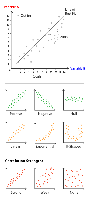
A scatter plot is a graphical representation that uses dots to represent the values obtained for two different variables - one plotted along the x-axis and the other plotted along the y-axis. Scatter plots are particularly useful for displaying the relationship between two continuous variables. Their uses include:
- Correlation Analysis: One of the primary uses of scatter plots is to observe correlations between variables. A positive correlation shows that as one variable increases, the other also does, whereas a negative correlation indicates that as one variable increases, the other decreases.
- Identify Trends: Scatter plots can reveal trends in your data, helping to identify different types of relationships among variables. Linear, exponential, and even non-functional trends can be observed.
- Outlier Detection: Scatter plots make it easy to spot outliers—data points that are significantly different from the others. These could be errors or important observations.
- Data Clustering: Sometimes, data points in scatter plots naturally form clusters, which can be valuable for classifying data into different categories.
- Multi-Dimensional Analysis: Scatter plots can be extended into “scatter plot matrices” or 3D scatter plots to visualize relationships among more than two variables.
- Comparisons: By overlaying scatter plots with different variables or subsets, you can make direct comparisons, which can be useful in A/B testing or time-series analysis.
5.4.1 Scatterplots in base R
Let’s start by creating a scatterplot of flipper length against body mass for the penguins dataset. We can do this using the plot() function:
# Scatterplot of flipper length against body mass
plot(penguins$flipper_length_mm,                          # Specify data
     penguins$body_mass_g,                                # Specify data
     main = "Scatterplot of Flipper Length vs Body Mass", # Add title
     xlab = "Flipper Length (mm)",                        # Add x-axis label
     ylab = "Body Mass (g)")                              # Add y-axis label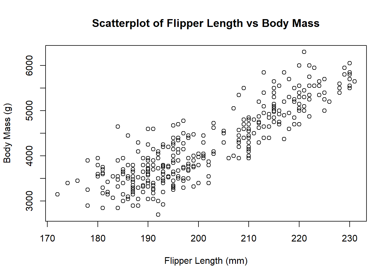
5.4.2 Scatterplots in ggplot2
We can create the same scatterplot using ggplot2:
# Create scatterplot of flipper length against body mass
ggplot(data = penguins, aes(x = flipper_length_mm, y = body_mass_g)) + # Specify data and aesthetic mappings
  geom_point() +                                                       # Add scatterplot layer
  labs(title = "Scatterplot of Flipper Length vs Body Mass",           # Add title
       x = "Flipper Length (mm)",                                      # Add x-axis label
       y = "Body Mass (g)")                                            # Add y-axis label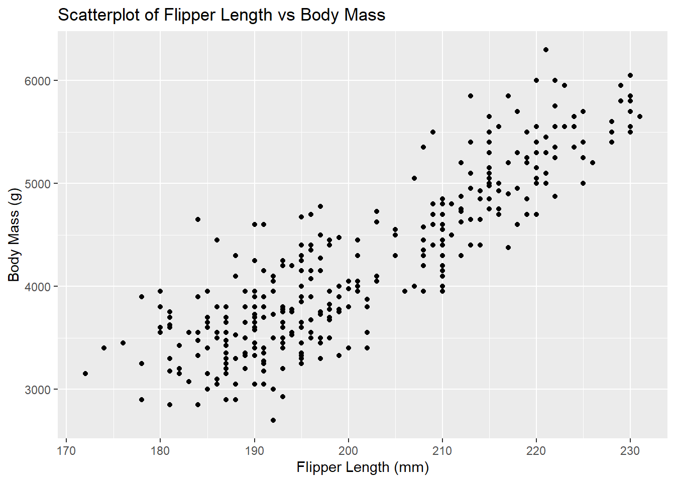
5.5 Lineplots
A lineplot is a type of graphical representation that uses lines to connect individual data points displayed along a numerical axis. The lines serve to show trends over a given time period or across categories, helping to visualize the relationship between two or more variables. Their uses include:
- Trend Analysis: One of the primary uses of lineplots is to visualize trends over time. For example, you could use a lineplot to show how stock prices or temperature have changed over the years.
- Comparing Multiple Series: lineplots allow for the comparison of multiple data series on the same chart, making it easier to observe relationships or disparities between different datasets.
- Frequency: In statistical analysis, lineplots can be used to visualize the frequency of data points, similar to histograms but for time-series or ordinal data.
- Prediction: The trends identified in lineplots can be useful for making predictions or forecasts about future data points.
- Data Relationships: They are also useful for showing the relationship between two variables, much like scatter plots, but with the added context of progression or time.
Unfortunately, the palmerpenguins data set does not contain time-related data so let’s simulate some data:
# Simulate new data
newdata <- data.frame(x = runif(24, -2, 2), # Create a variable x with 24 values between -2 and 2
                      y = rnorm(24))        # Create a variable y with 24 random normal values
5.5.1 Lineplots in base R
Let’s start by creating a lineplot of the simulated data. We can do this using the plot() function:
# Create a basic scatterplot
plot(y ~ x,            # Specify data
     data = newdata,   # Specify data
     pch = 16,         # Specify point symbol
     col = "blue")     # Specify point colour

# Add a line to the scatterplot
lines(y[order(x)] ~ x[order(x)], # Specify data and order it by variable x
      data = newdata,            # Specify data
      col = "red")               # Specify line colour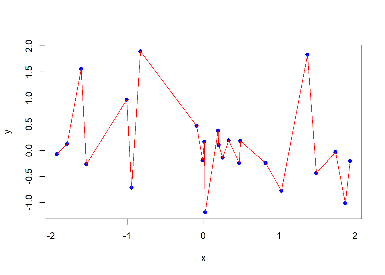
You can also draw a lineplot without the points:
# Eliminate the points, and some options
plot(y[order(x)] ~ x[order(x)],      # Specify data and order it by variable x
     data = newdata, type = "l",     # Specify data and line type
     lty = 3, lwd = 2, col = "red")  # Specify line type, width and colour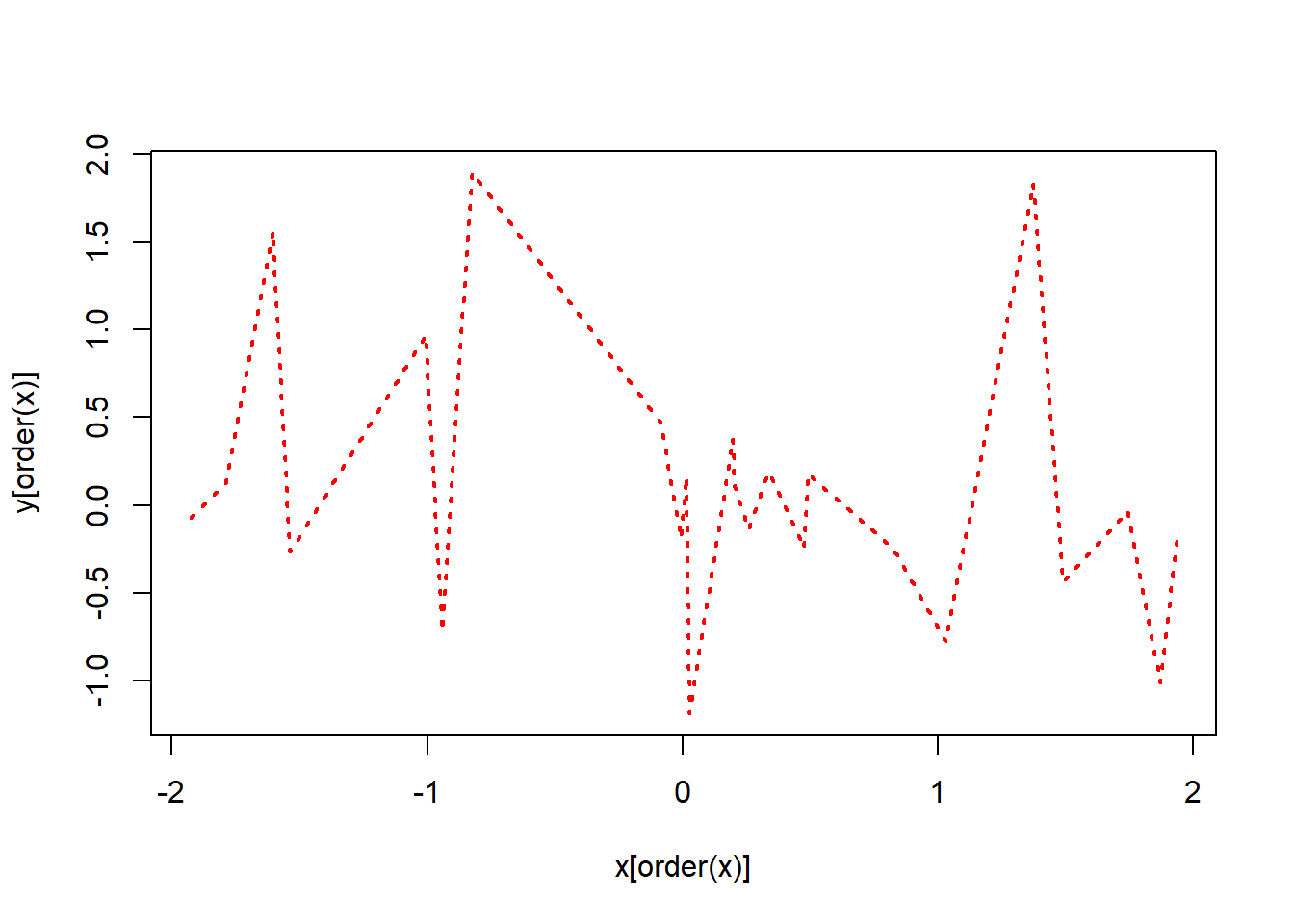
5.5.2 Lineplots in ggplot2
We can create the same lineplot using ggplot2:
# Create lineplot
ggplot(data = newdata, aes(x = x, y = y)) +  # Specify data and aesthetic mappings
  geom_point() +                             # Add scatterplot layer
  geom_line() +                              # Add line layer
  labs(title = "Lineplot",                   # Add title
       x = "X",                              # Add x-axis label
       y = "Y")                              # Add y-axis label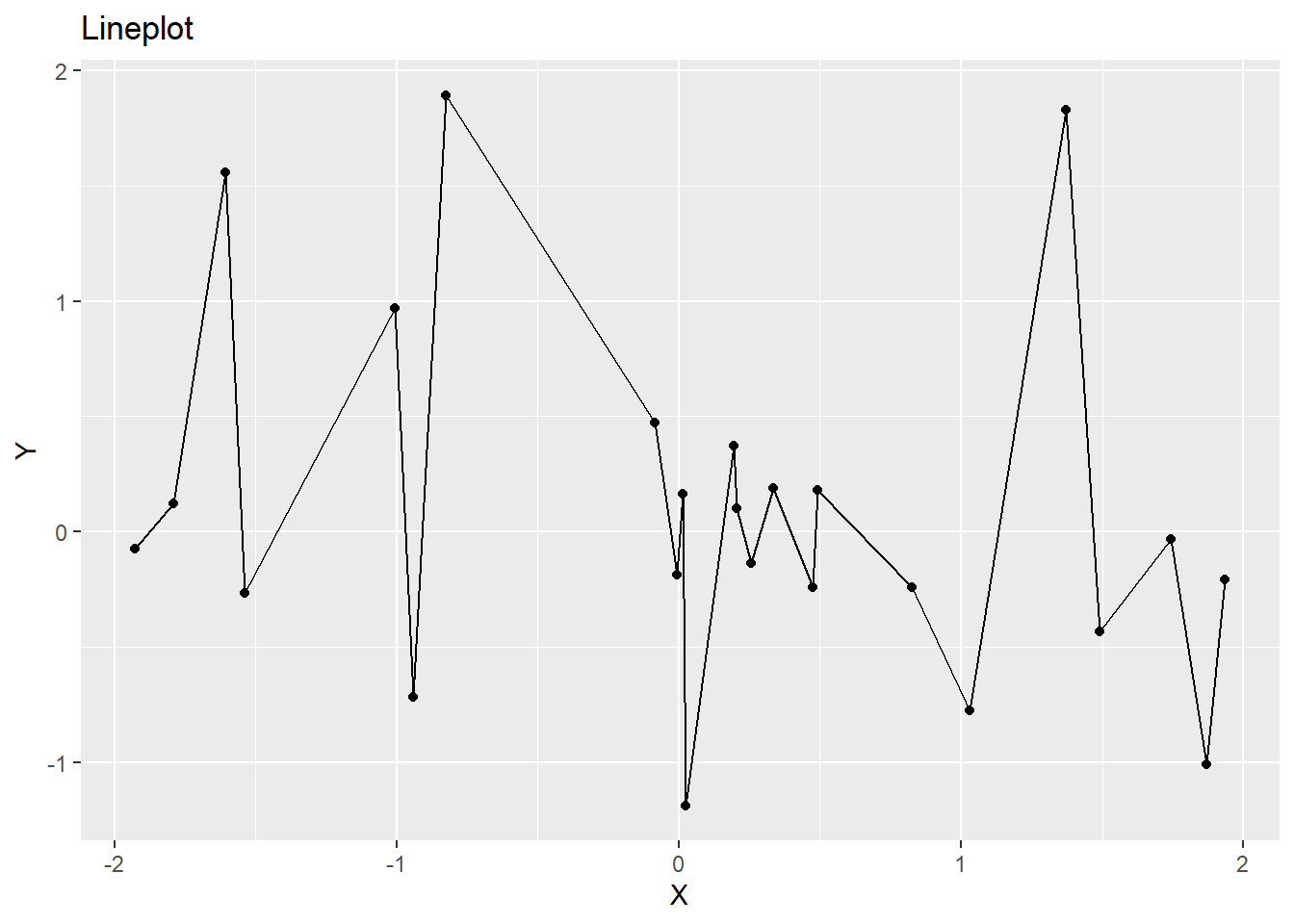
You can also draw a lineplot without the points:
# Create lineplot
ggplot(data = newdata, aes(x = x, y = y)) +  # Specify data and aesthetic mappings
  geom_line(colour = "red") +                # Add line layer
  labs(title = "Lineplot",                   # Add title
       x = "X",                              # Add x-axis label
       y = "Y")                              # Add y-axis label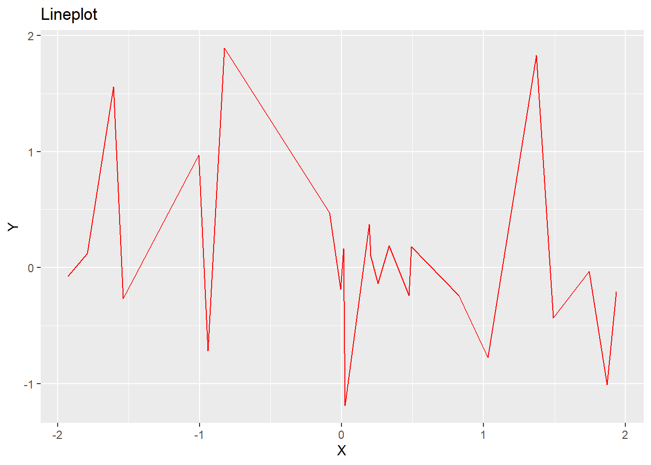
6 Lattice Graphs
Lattice graphics is a powerful and elegant high-level data visualization system that is included in the R programming language. It is inspired by and based on the trellis graphics package developed by Richard Becker, William Cleveland and Allan Wilks. Lattice graphics is implemented in the lattice package and is a part of base R. Let’s go ahead and install and load the lattice package:
# Check whether a package is installed and install if not
if(!require("lattice")) install.packages("lattice")
Loading required package: lattice# Load the lattice package
library(lattice, quietly = TRUE)6.1 Lattice Functions
The lattice package contains a number of functions that can be used to create different types of plots. The most commonly used functions are:
histogram(): Used to create histograms;bwplot(): Used to create boxplots;barchart(): Used to create barplots;xyplot(): Used to create scatterplots and lineplots.
Let’s go ahead and recreate the plots we created in the previous section using lattice graphics.
6.2 Histograms
# Create histogram
histogram(~ flipper_length_mm,           # Specify data
          data = penguins,               # Specify data
          main = "Histogram",            # Add title
          xlab = "Flipper Length (mm)",  # Add x-axis label
          ylab = "Frequency")            # Add y-axis label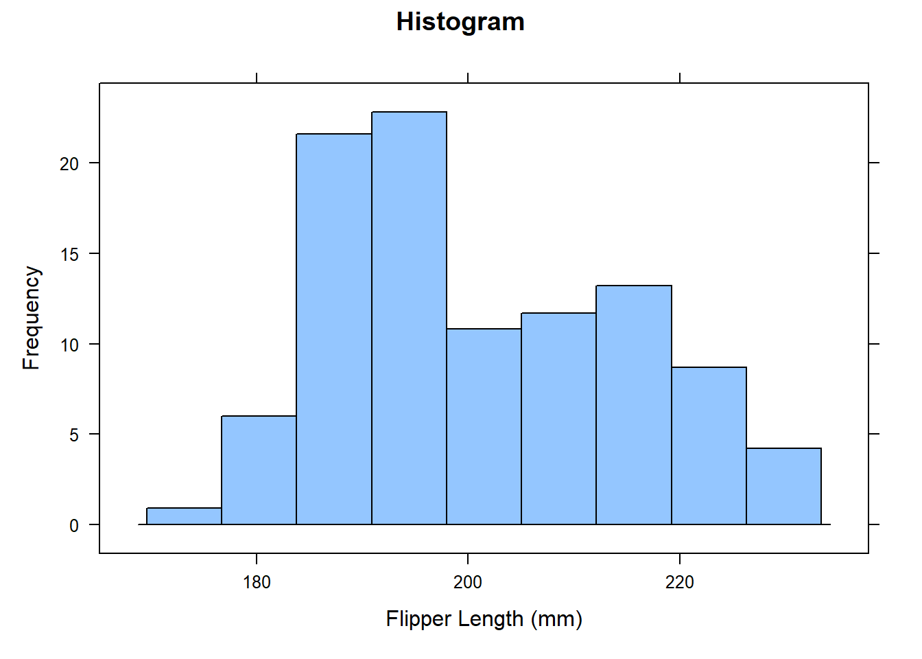
6.3 Boxplots
# Create boxplot
bwplot(species ~ flipper_length_mm,   # Specify data
       data = penguins,               # Specify data
       main = "Boxplot",              # Add title
       xlab = "Flipper Length (mm)",  # Add x-axis label
       ylab = "Species")              # Add y-axis label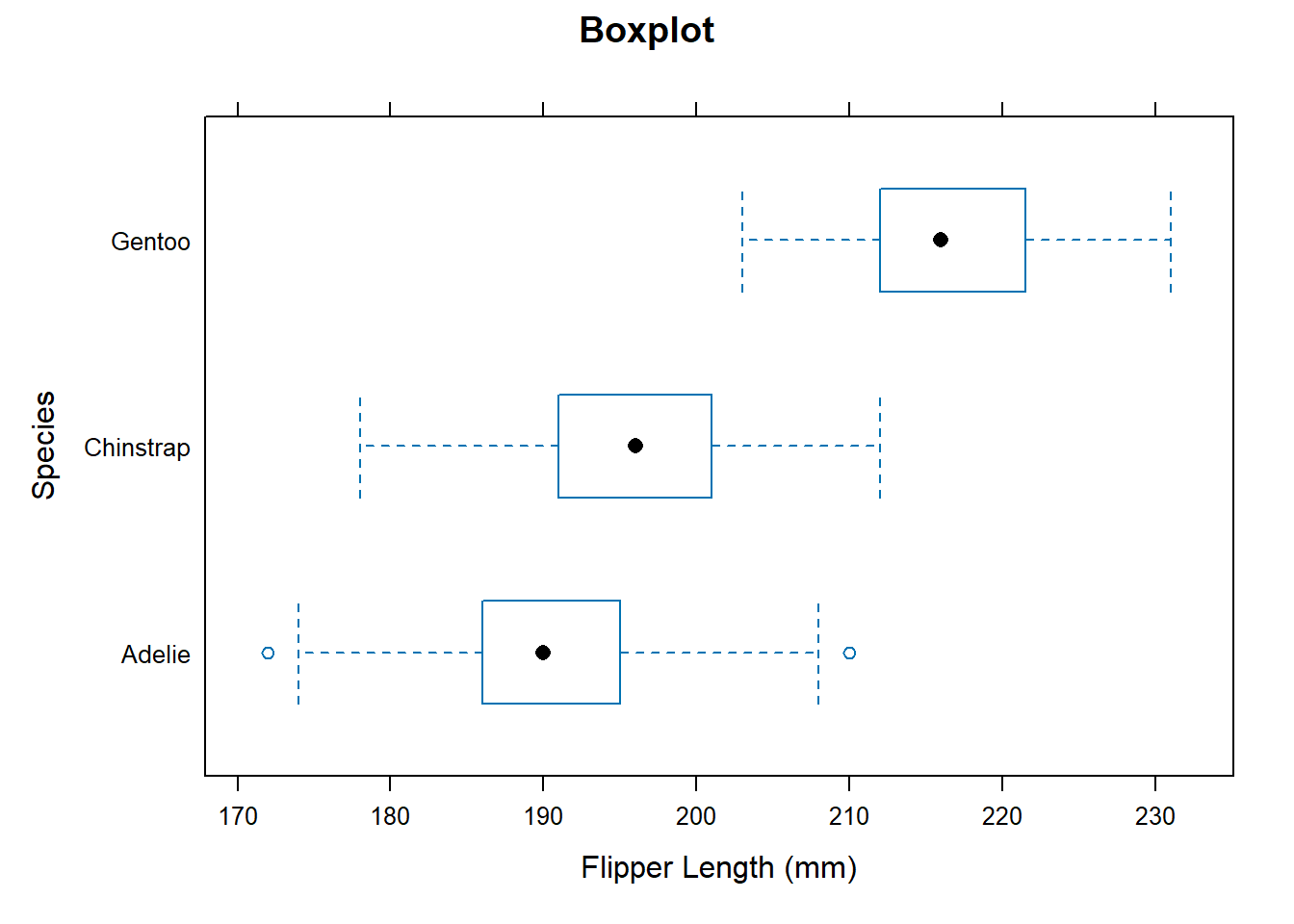
6.4 Barplots
# Create barplot
barchart(species ~ flipper_length_mm,   # Specify data
         data = penguins,               # Specify data
         main = "Barplot",              # Add title
         xlab = "Flipper Length (mm)",  # Add x-axis label
         ylab = "Species")              # Add y-axis label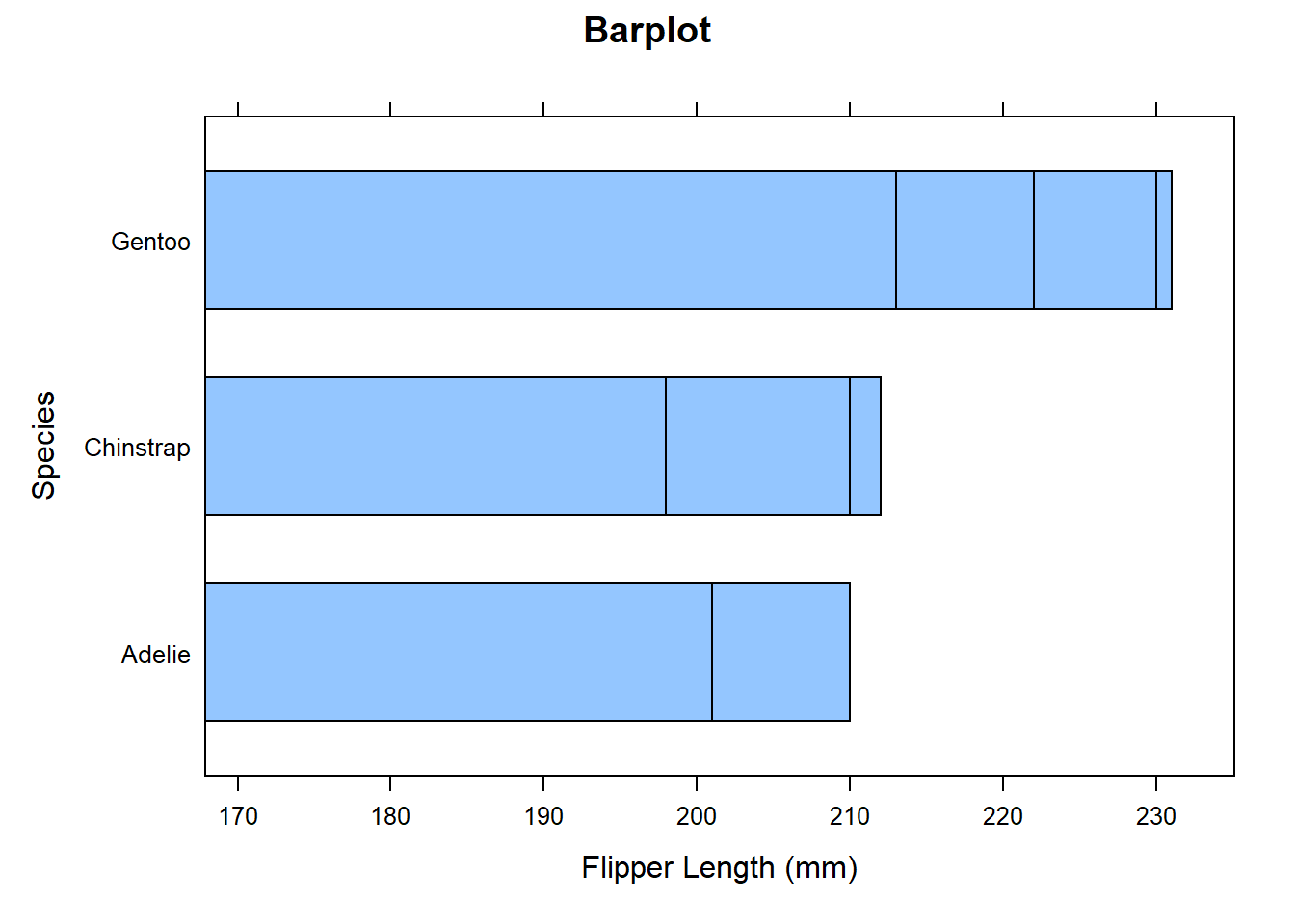
6.5 Scatterplots
# Create scatterplot
xyplot(flipper_length_mm ~ body_mass_g,  # Specify data
       data = penguins,                  # Specify data
       main = "Scatterplot",             # Add title
       xlab = "Body Mass (g)",           # Add x-axis label
       ylab = "Flipper Length (mm)")     # Add y-axis label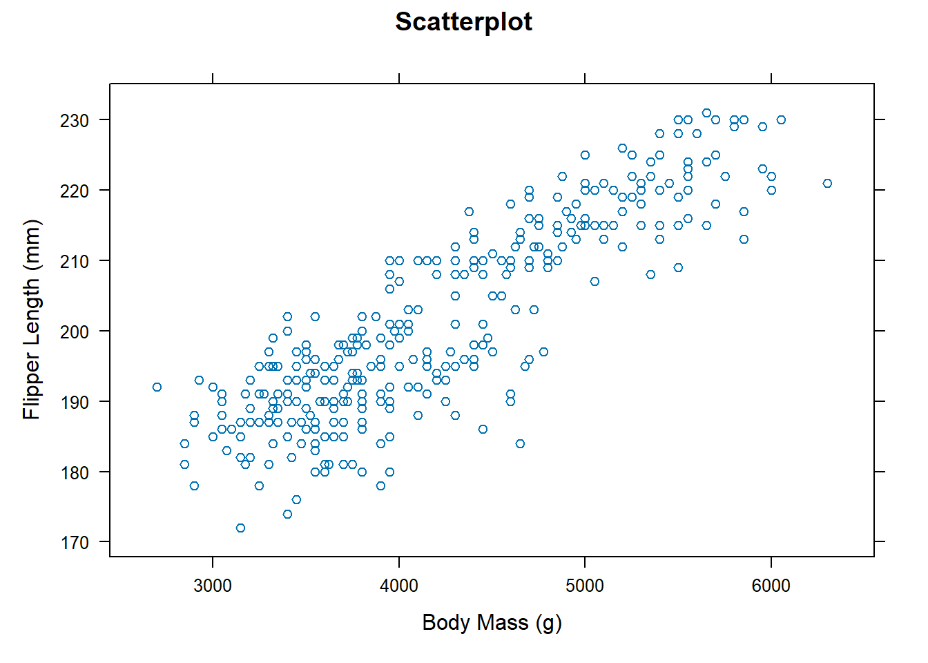
Let’s add a regression line to the scatterplot and colour the points by species:
# Create scatterplot
xyplot(flipper_length_mm ~ body_mass_g,  # Specify data
       data = penguins,                  # Specify data
       main = "Scatterplot",             # Add title
       xlab = "Body Mass (g)",           # Add x-axis label
       ylab = "Flipper Length (mm)",     # Add y-axis label
       type = c("p", "r"),               # Add points and regression line
       groups = species,                 # Colour points by species
       auto.key = list(space = "right",  # Add legend
                       columns = 1))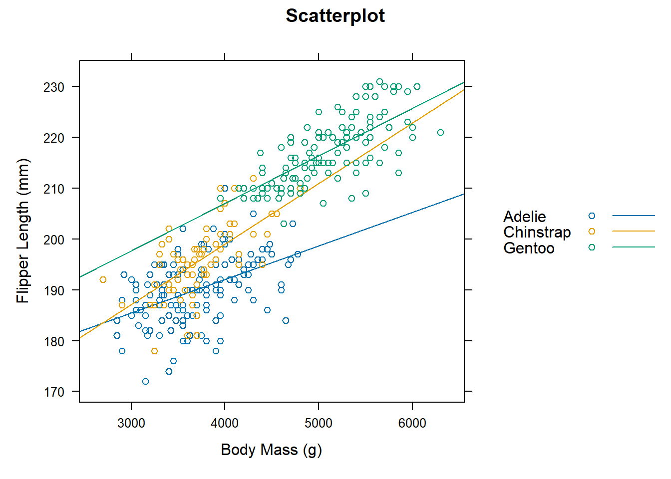
Lattice isn’t as flexible as ggplot2 but it is very powerful and can be used to create a wide variety of plots. For more information on lattice graphics, check out the official documentation.
7 Choosing Graphs
The process of deciding what type of data visualisation to create begins with a simple question: Why am I doing this? Data visualisations must serve a purpose so all decisions about chart type, design, layout, and more, should flow from a clear understanding of the intended purpose of a graphic. I suggest working through the following questions to help you determine what type of visualisation you should create for your data:
- Is the aim of the graph to find something out (“analysis graph”), or to make a point to others?
- What do you want to find out?
- Who is the audience for the graph?
Identifying the target audience at an early stage is crucial, as different groups of people are likely to have different levels of graph literacy depending on their education level, technical expertise, prior exposure to data visualisation formats, and other factors. Design decisions that do not properly account for the needs of the intended audience will fail to achieve their aims.
Once you have answered these questions, you can start to think about what type of graph you should create. The following table provides a summary of the different types of some common graphs and when you should use them:
| Graph Type | When to Use |
|---|---|
| Bar Chart | To compare values across categories |
| Histogram | To show the distribution of a numerical variable |
| Boxplot | To show the distribution of a numerical variable |
| Scatterplot | To show the relationship between two numerical variables |
| Line Chart | To show the relationship between two numerical variables over time |
| Pie Chart | To show the proportion of a whole |
| Heatmap | To show the relationship between two categorical variables |
| Map | To show the relationship between numerical variables geographically |
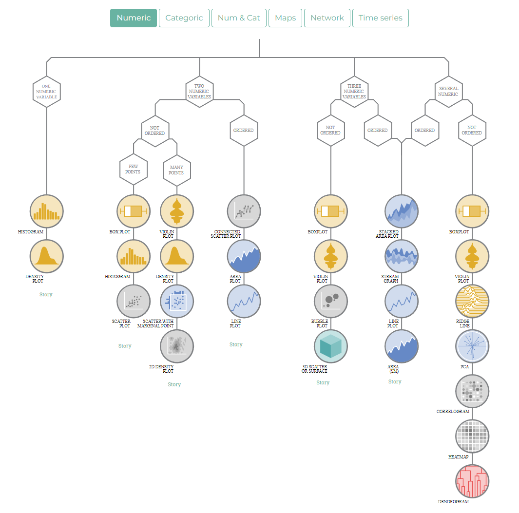
There are, however, a range of online tools to help you decide on the best type of graph for your data. For example, the Data Viz Project provides a searchable database of different types of graphs and when to use them. From Data to Viz also provides a decision tree to help you decide on the best type of graph for your data:
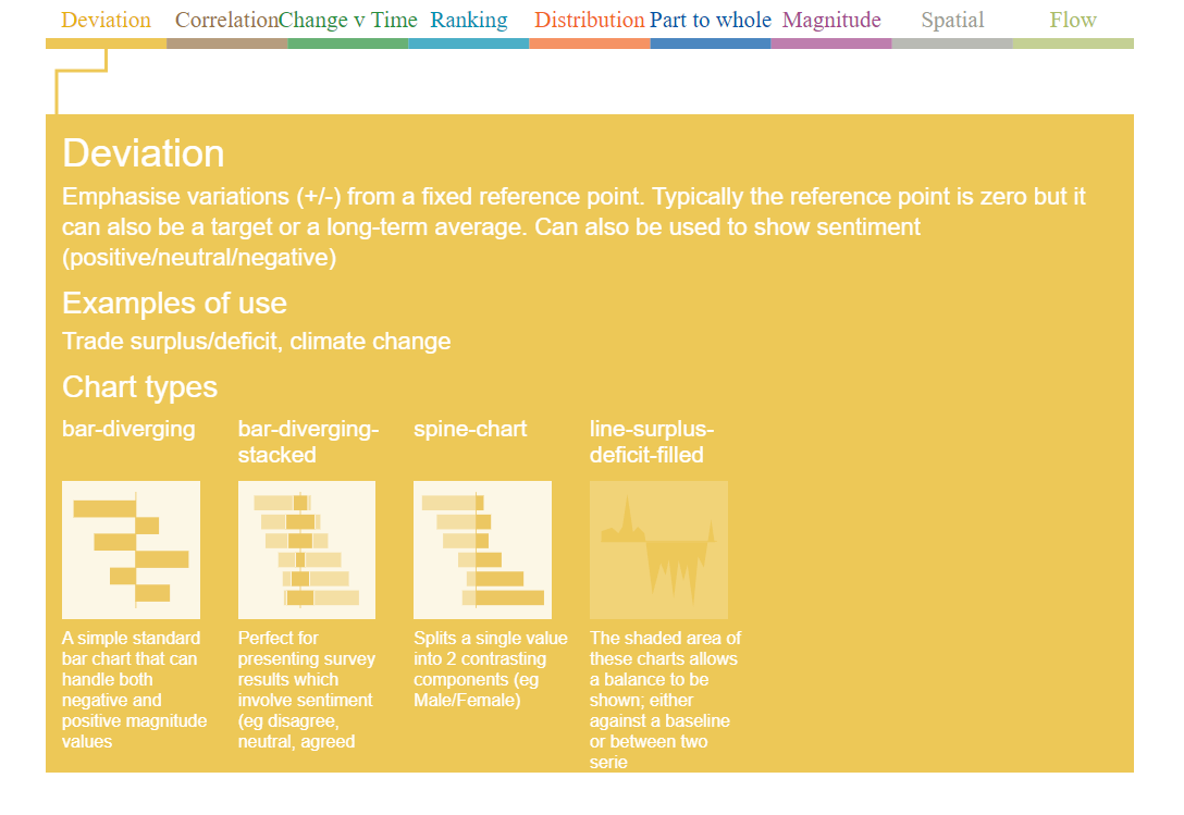
Visual Vocabulary is a site developed by the data visualisation team at the Financial Times. It allows users to narrow down the choice of chart type based on the data relationship that is “most important in your story”. Relationship options include deviation, correlation, change versus time, ranking, and more.
8 Activities
Let’s use the data from an R package called mtcars to practice creating different types of plots. The mtcars dataset contains fuel consumption and 10 aspects of automobile design and performance for 32 automobiles (1973-74 models). The first thing you should do is load this dataset using the following code:
# Load the mtcars data
data(mtcars)
8.1 Variables
Using the new skills you have learned on Monday, inspect this dataset to determine whether the data are tidy and what type of variables you are working with.
💡 Click here to view a solution
# Inspect the mtcars data
glimpse(mtcars)
You will note that the vehicle name is not a variable in this dataset. This is because the vehicle name is used as the row name. This will be a problem when it comes to plotting the data! To convert the row name into a variable, you can use the rownames_to_column() function from the tibble package:
# Convert row name to variable
mtcars <- tibble::rownames_to_column(mtcars,               # Specify data
                                     var = "vehicle_name") # Specify variable name
8.2 Create a histogram
Create a histogram of the mpg variable using Base R and then describe the distribution of the variable.
💡 Click here to view a solution
# Create a histogram of the mpg variable
hist(mtcars$mpg,                # Specify variable
     main = "Histogram of MPG", # Add title
     xlab = "Miles per Gallon", # Add x-axis label
     ylab = "Frequency",        # Add y-axis label
     breaks = 10)               # Specify number of bins
This distribution is unimodal (one-peak) and slightly skewed to the right. The majority of cars in this dataset have a fuel consumption of between 15 and 20 miles per gallon.
8.3 Create a boxplot
Create a boxplot of the mpg variable using ggplot2. What is the median fuel consumption of the cars in this dataset?
💡 Click here to view a solution
# Create a boxplot of the mpg variable
ggplot(data = mtcars, aes(x = "", y = mpg)) +  # Specify data and aesthetic mappings
  geom_boxplot() +                             # Add boxplot layer
  labs(title = "Boxplot of MPG",               # Add title
       x = "",                                 # Remove x-axis label
       y = "Miles per Gallon")                 # Add y-axis label
The median fuel consumption of the cars in this dataset is 19.2 miles per gallon. You can also calculate this value using the median() function:
# Calculate the median fuel consumption
median(mtcars$mpg)
8.4 Create a scatterplot
Create a scatterplot of the mpg and wt variables using lattice. Describe the relationship between the two variables and add a regression line.
💡 Click here to view a solution
# Create a scatterplot of the mpg and wt variables
xyplot(mpg ~ wt, data = mtcars,                 # Specify data and variables
       main = "Scatterplot of MPG and Weight",  # Add title
       xlab = "Weight",                         # Add x-axis label
       ylab = "Miles per Gallon")               # Add y-axis label
This scatterplot shows a negative linear relationship between fuel consumption and weight. As the weight of the car increases, the fuel consumption decreases.
To add a regression line to this plot, you can use the panel.lmline() function from the latticeExtra package:
# Add regression line to scatterplot
xyplot(mpg ~ wt, data = mtcars,  # Specify data and variables
       main = "Scatterplot of MPG and Weight",  # Add title
       xlab = "Weight",                        # Add x-axis label
       ylab = "Miles per Gallon",              # Add y-axis label
       panel = function(x, y, ...) {
         panel.xyplot(x, y, ...)              # Add scatterplot layer
         panel.lmline(x, y, col = "red")      # Add regression line layer
       })
9 Recap
- Data visualisation is the graphical representation of data and information;
- Data visualisation is important because it allows us to communicate information clearly and efficiently;
- There are many different types of graphs that can be used to visualise data;
- The type of graph you choose will depend on the type of data you are working with and the story you are trying to tell;
- The
ggplot2package is a powerful tool for creating data visualisations inR.