# Load packages
library(tidyverse)
library(palmerpenguins)
library(gridExtra)
library(patchwork)
library(cowplot)

# Load data
data(penguins)

# Filter data to remove missing values
penguins <- penguins %>%
filter(!is.na(flipper_length_mm), !is.na(body_mass_g)) Multi-Panel Plotting
R
Set Up R Environment
Create Two Basic Plots
Plot 1 - Scatterplot
# Create a scatterplot of flipper length against body mass for each species
plot_1 <- ggplot(data = penguins, aes(                    # Set data and aesthetics
  x = flipper_length_mm,                                  # Set x-axis variable
  y = body_mass_g,                                        # Set y-axis variable
  colour = species                                        # Set colour variable
)) +
  geom_point() +                                          # Add points
  labs(
    title = "Scatterplot of Flipper Length vs Body Mass", # Add title
    x = "Flipper Length (mm)",                            # Add x-axis label
    y = "Body Mass (g)",                                  # Add y-axis label
    colour = "Species"                                    # Add legend title
  ) +
  theme(legend.position = "bottom")                       # Move legend to bottom

# View plot
plot_1 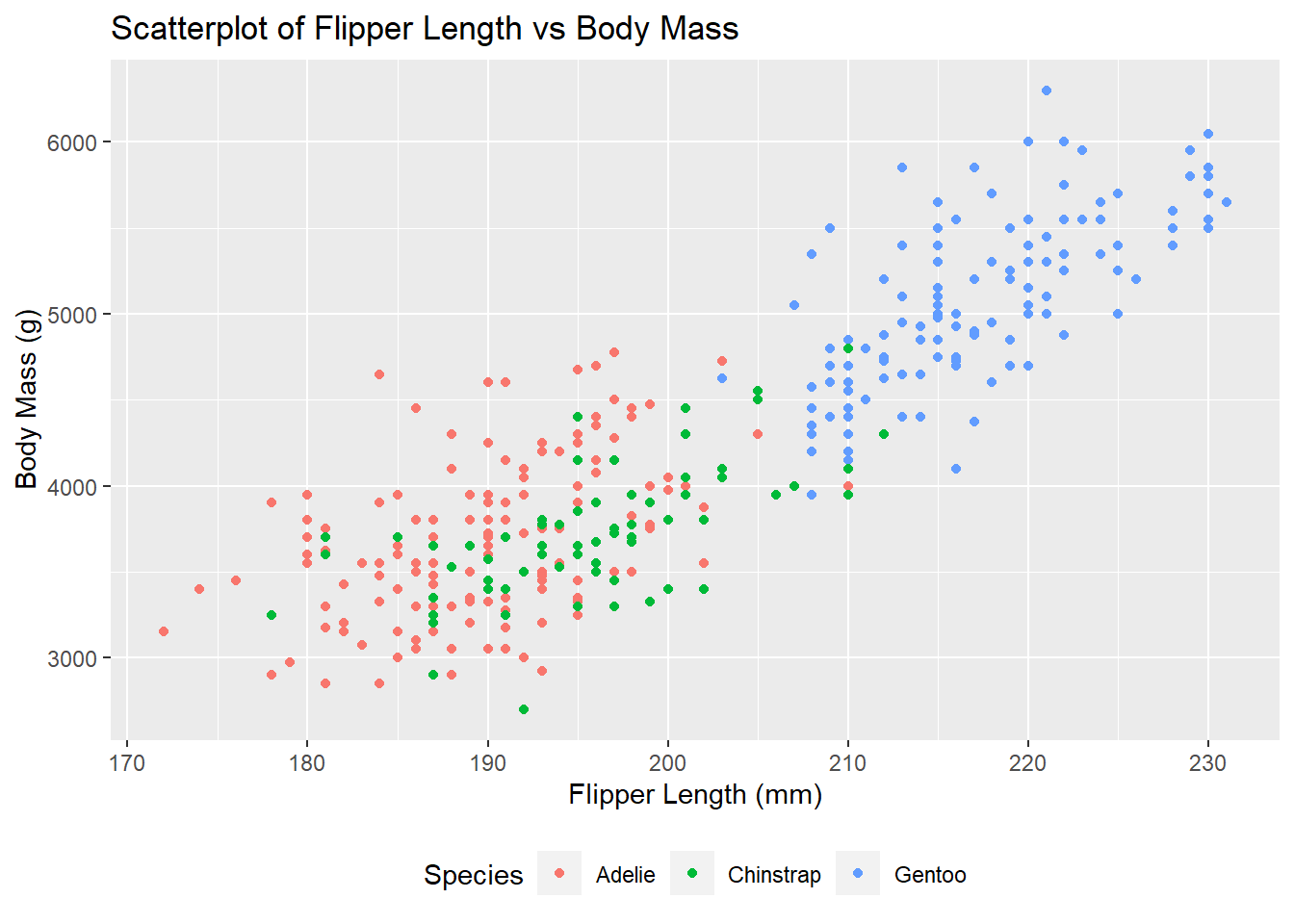
Plot 2 - Histogram
# Create a histogram of flipper length for each species
plot_2 <- ggplot(data = penguins, aes(     # Set data and aesthetics
  x = flipper_length_mm,                   # Set x-axis variable
  fill = species                           # Set fill variable
)) +
  geom_histogram() +                       # Add histogram
  labs(
    title = "Histogram of Flipper Length", # Add title
    x = "Flipper Length (mm)",             # Add x-axis label
    y = "Count",                           # Add y-axis label
    fill = "Species"                       # Add legend title
  ) +
  theme(legend.position = "bottom")        # Move legend to bottom

# View plot
plot_2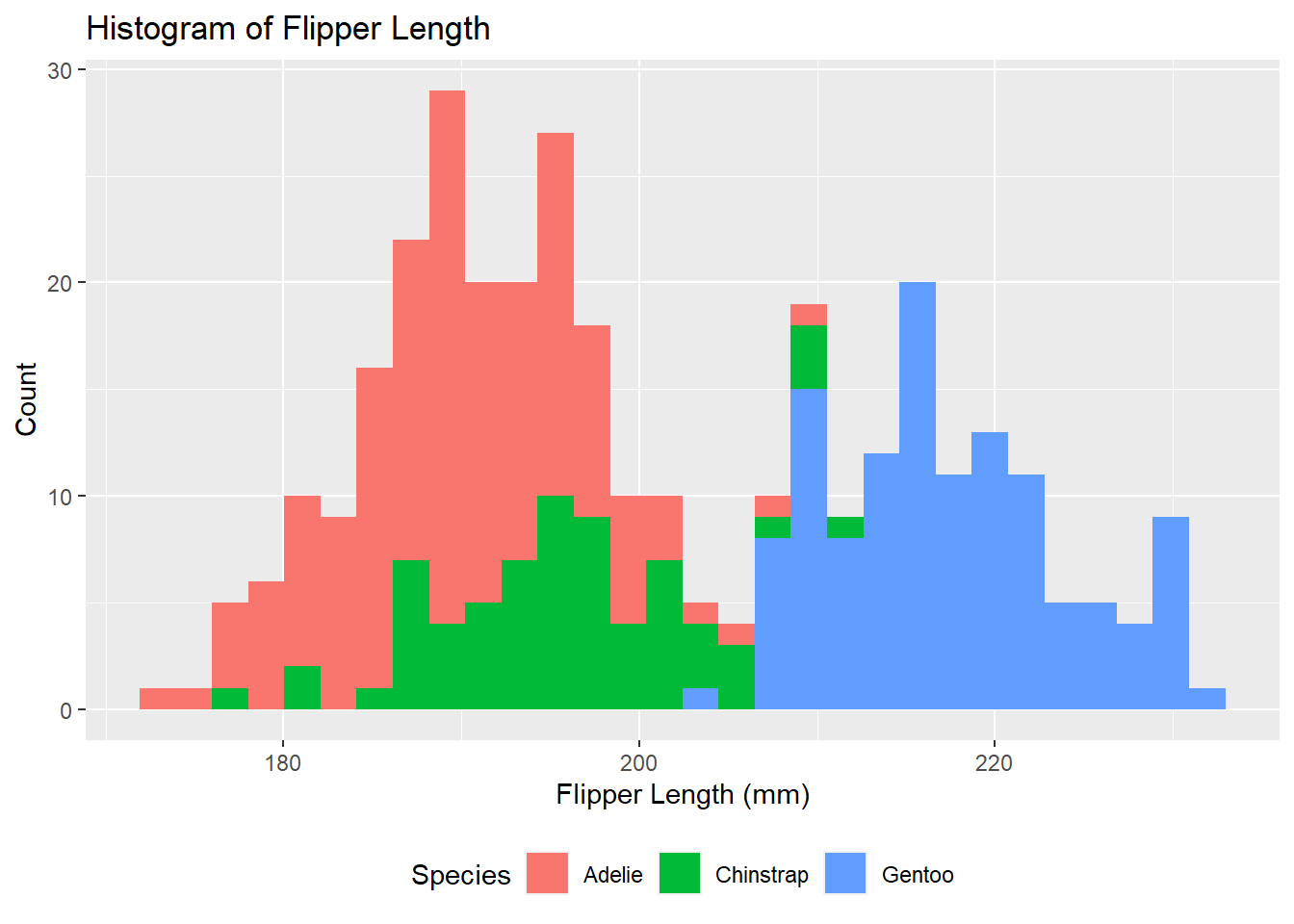
Plot 3 - Boxplot
# Create a boxplot of flipper length for each species
plot_3 <- ggplot(data = penguins, aes(   # Set data and aesthetics
  x = species,                           # Set x-axis variable
  y = flipper_length_mm,                 # Set y-axis variable
  fill = species                         # Set fill variable
)) +
  geom_boxplot() +                       # Add boxplot
  labs(
    title = "Boxplot of Flipper Length", # Add title
    x = "Species",                       # Add x-axis label
    y = "Flipper Length (mm)",           # Add y-axis label
    fill = "Species"                     # Add legend title
  ) +
  theme(legend.position = "bottom") +    # Move legend to bottom
  coord_flip()                           # Flip x- and y-axes

# View plot
plot_3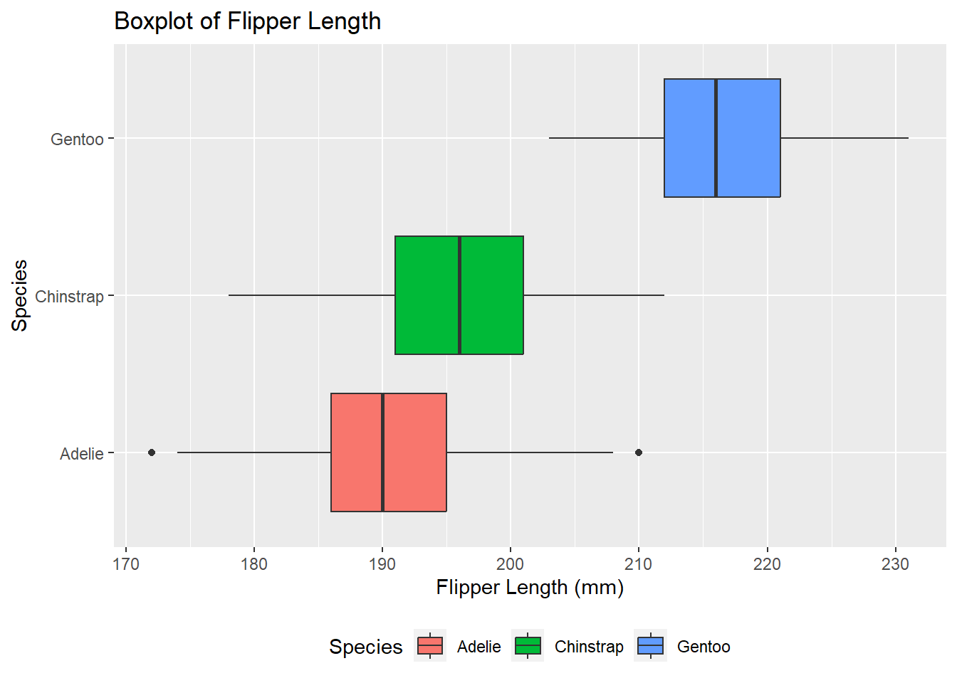
Combine Plots
gridExtra
More info here.
# Plot two plots side-by-side
grid.arrange(plot_1,   # Plot 1
             plot_2,   # Plot 2
             ncol = 2) # Number of columns
# Plot two plots above each other
grid.arrange(plot_1,   # Plot 1
             plot_2,   # Plot 2
             nrow = 2) # Number of rows
# Plot three plots in a 1x3 grid
grid.arrange(plot_1,   # Plot 1
             plot_2,   # Plot 2
             plot_3,   # Plot 3
             ncol = 3) # Number of columns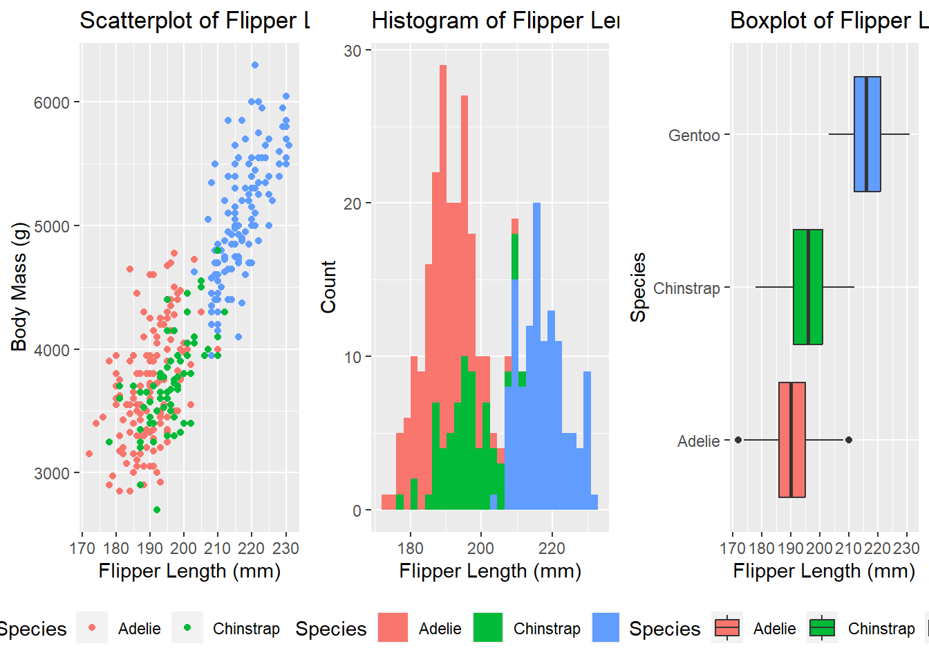
# Plot three plots in a 3x1 grid
grid.arrange(plot_1,   # Plot 1
             plot_2,   # Plot 2
             plot_3,   # Plot 3
             nrow = 3) # Number of rows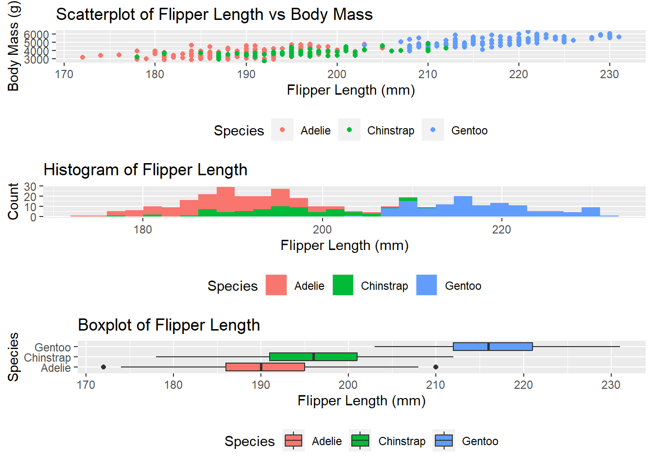
patchwork
More info here.
# Plot these two plots side-by-side
plot_1 + plot_2 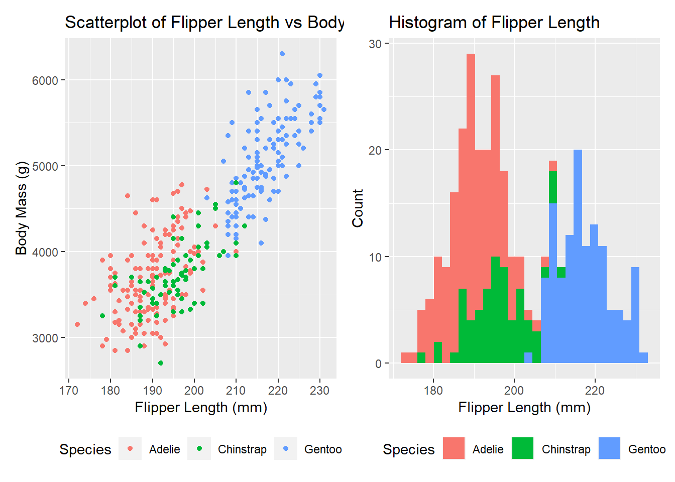
# Plot these two plots above each other
plot_1 / plot_2 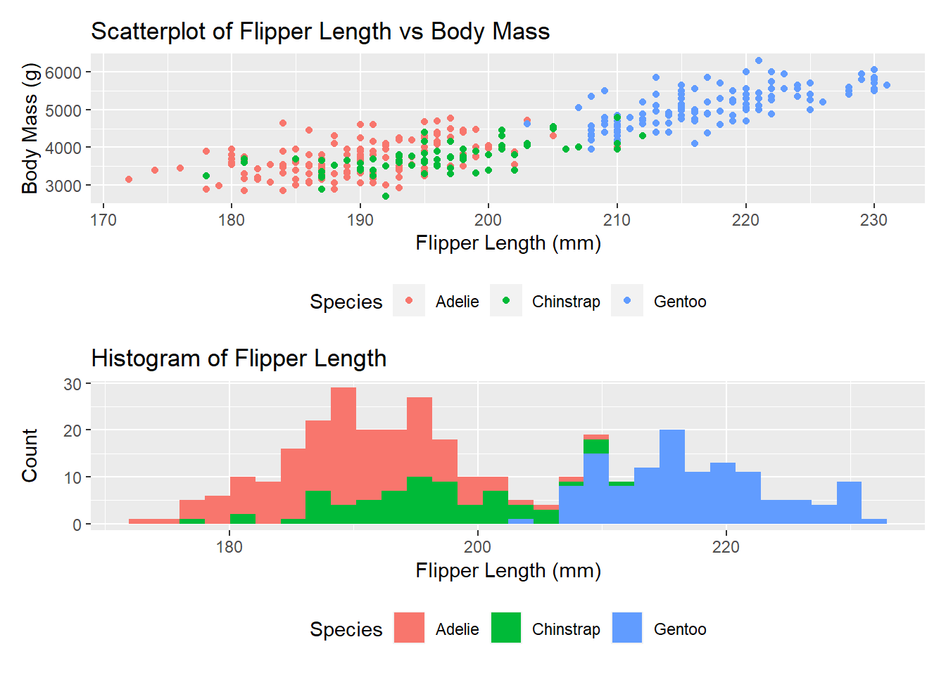
# Plot two plots on top and one plot on bottom
(plot_1 | plot_2) / plot_3 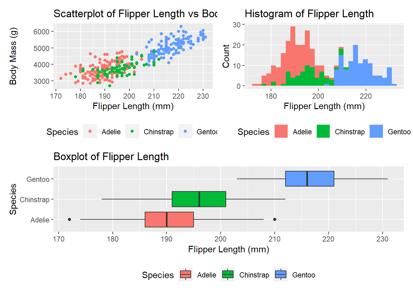
cowplot
More info here.
# Plot these two plots side-by-side using cowplot
plot_grid(plot_1,       # Plot 1
          plot_2,       # Plot 2
          ncol = 2,     # Number of columns
          scale = TRUE) # Scale plots to same size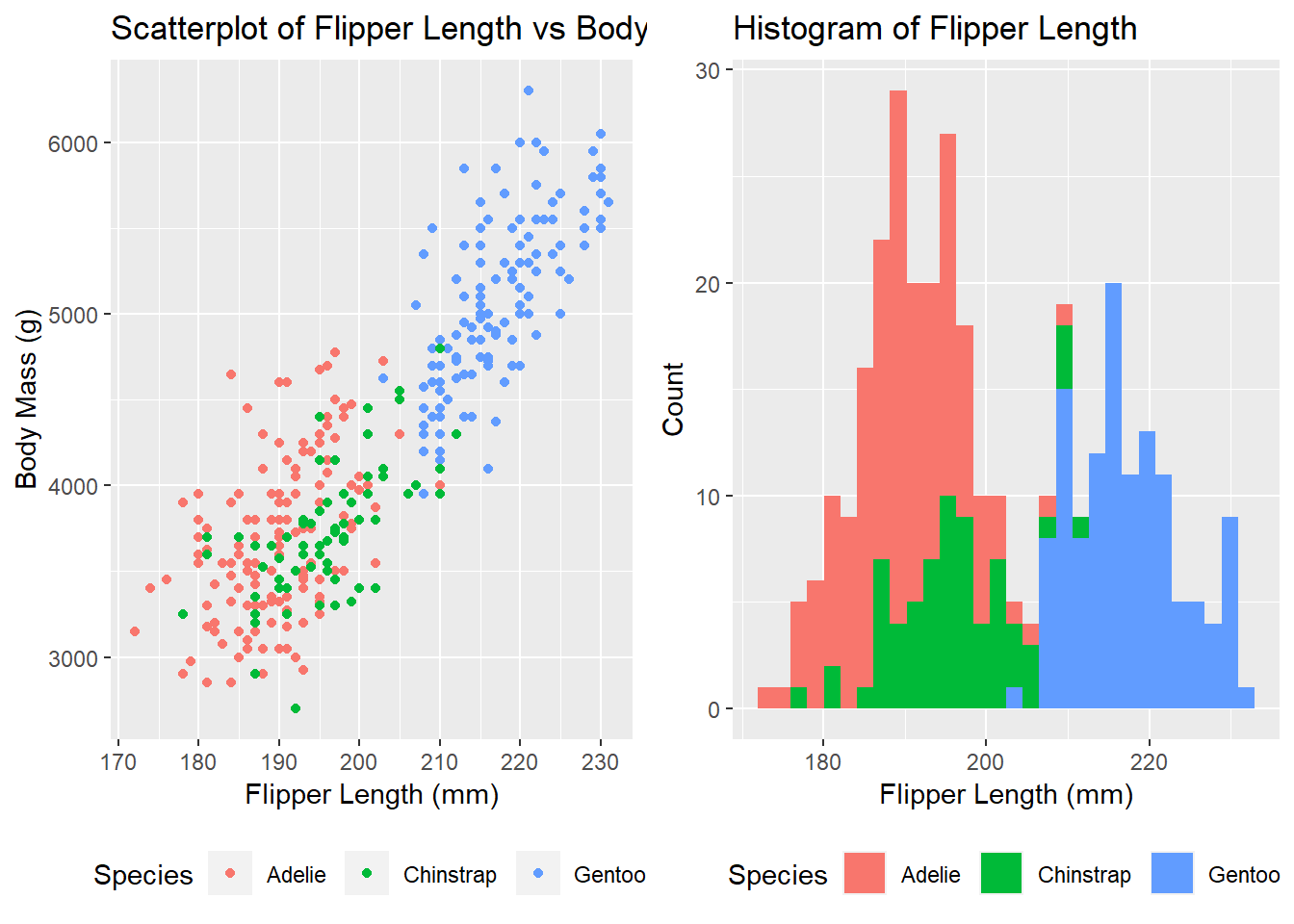
# Plot these two plots above each other using cowplot
plot_grid(plot_1,       # Plot 1
          plot_2,       # Plot 2
          nrow = 2,     # Number of rows
          scale = TRUE) # Scale plots to same size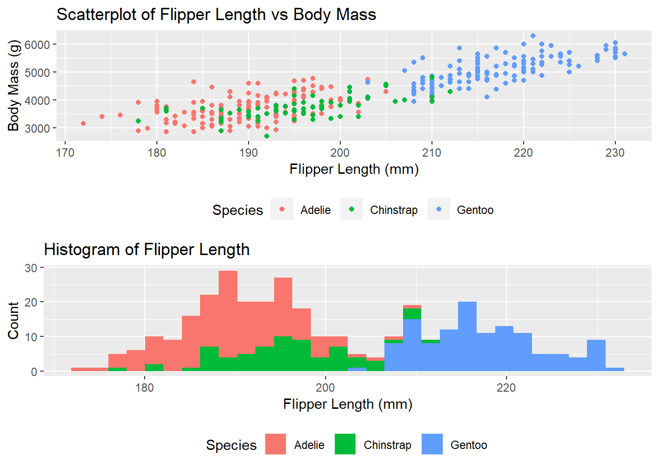
Python
Set Up Python Environment
# Load packages
import pandas as pd
import numpy as np
import matplotlib.pyplot as plt
import seaborn as sns
import matplotlib.gridspec as gridspec

# Read in data
penguins = pd.read_csv("https://raw.githubusercontent.com/allisonhorst/palmerpenguins/master/inst/extdata/penguins.csv")

# Filter data to remove missing values
penguins = penguins.dropna(subset = ["flipper_length_mm", "body_mass_g"])
Combine Plots
gridspec
# Create figure and axis objects
fig = plt.figure(constrained_layout=True) # Ensures that the subplots fit within the figure

# Create grid with 1 row and 2 columns
gs = fig.add_gridspec(1, 2) # 1 row, 2 columns

# Add plots to grid
ax1 = fig.add_subplot(gs[0, 0]) # First row, first column

ax2 = fig.add_subplot(gs[0, 1]) # First row, second column

# Scatter plot
sns.scatterplot(data=penguins,                 # Set data
                        x="body_mass_g",       # Set x-axis variable
                        y="flipper_length_mm", # Set y-axis variable
                        hue="species",         # Set colour variable
                        ax=ax1)                # Add plot to first subplot

# Add title and axis labels
ax1.set_title("Scatter plot of flipper length against body mass") # Add title
ax1.set_xlabel("Body mass (g)")                                   # Add x-axis label
ax1.set_ylabel("Flipper length (mm)")                             # Add y-axis label

# Histogram
sns.histplot(data=penguins,                  # Set data
                      x="flipper_length_mm", # Set x-axis variable
                      hue="species",         # Set colour variable
                      ax=ax2)                # Add plot to second subplot

# Add title and axis labels
ax2.set_title("Histogram of flipper length") # Add title
ax2.set_xlabel("Flipper length (mm)")        # Add x-axis label
ax2.set_ylabel("Count")                      # Add y-axis label

# Adjusts the subplots to fit into the figure area
plt.tight_layout()

# Show plot
plt.show()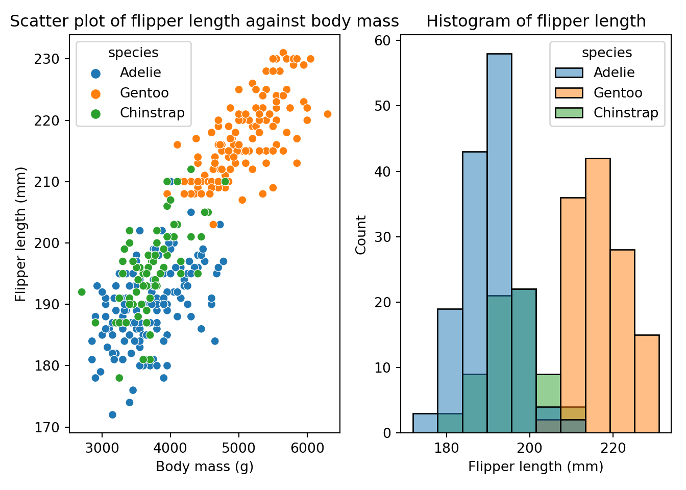
subplots
# Create a 1x2 grid of subplots
fig, (ax1, ax2) = plt.subplots(1, 2, figsize=(12, 6))  # 1 row, 2 columns

# Scatter plot on the first subplot
sns.scatterplot(data=penguins,         # Set data
                x="body_mass_g",       # Set x-axis variable
                y="flipper_length_mm", # Set y-axis variable
                hue="species",         # Set colour variable
                ax=ax1)                # Add plot to first subplot

# Add title and axis labels
ax1.set_title("Scatter plot of flipper length against body mass")
ax1.set_xlabel("Body mass (g)")
ax1.set_ylabel("Flipper length (mm)")

# Histogram on the second subplot
sns.histplot(data=penguins,            # Set data
             x="flipper_length_mm",    # Set x-axis variable
             hue="species",            # Set colour variable
             ax=ax2)                   # Add plot to second subplot

# Add title and axis labels
ax2.set_title("Histogram of flipper length")
ax2.set_xlabel("Flipper length (mm)")
ax2.set_ylabel("Count")

# Adjusts the subplots to fit into the figure area
plt.tight_layout()

# Show the plots
plt.show()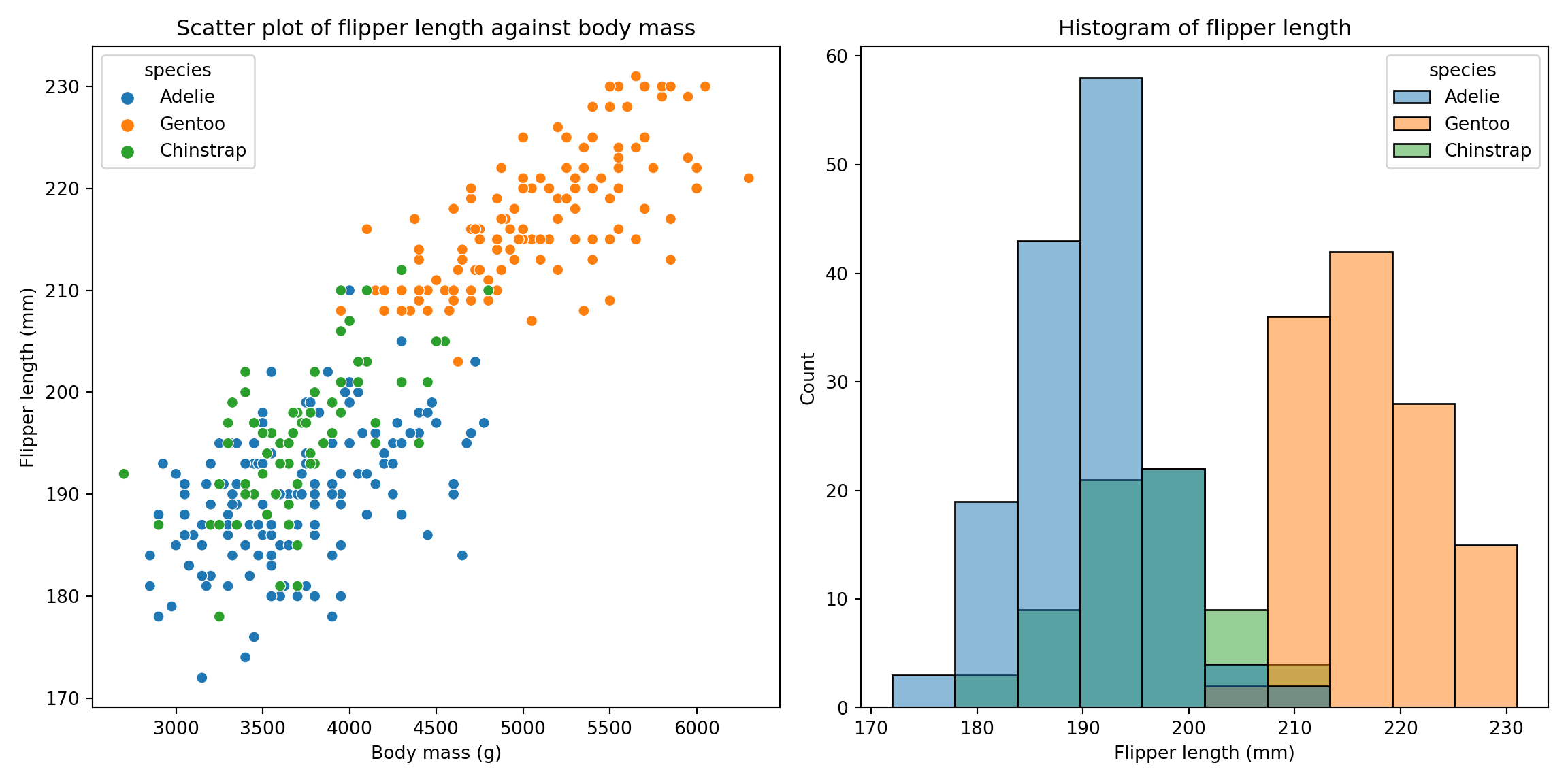
# Create a 1x3 grid of subplots
fig, (ax1, ax2, ax3) = plt.subplots(1, 3, figsize=(18, 6)) # 1 row, 3 columns
# Scatter plot on the first subplot
sns.scatterplot(data=penguins, # Set data
x="body_mass_g", # Set x-axis variable
y="flipper_length_mm", # Set y-axis variable
hue="species", # Set colour variable
ax=ax1) # Add plot to first subplot
# Add title and axis labels
ax1.set_title("Scatter plot of flipper length against body mass") # Add title
ax1.set_xlabel("Body mass (g)") # Add x-axis label
ax1.set_ylabel("Flipper length (mm)") # Add y-axis label
# Histogram on the second subplot
sns.histplot(data=penguins, # Set data
x="flipper_length_mm", # Set x-axis variable
hue="species", # Set colour variable
ax=ax2) # Add plot to second subplot
# Add title and axis labels
ax2.set_title("Histogram of flipper length") # Add title
ax2.set_xlabel("Flipper length (mm)") # Add x-axis label
ax2.set_ylabel("Count") # Add y-axis label
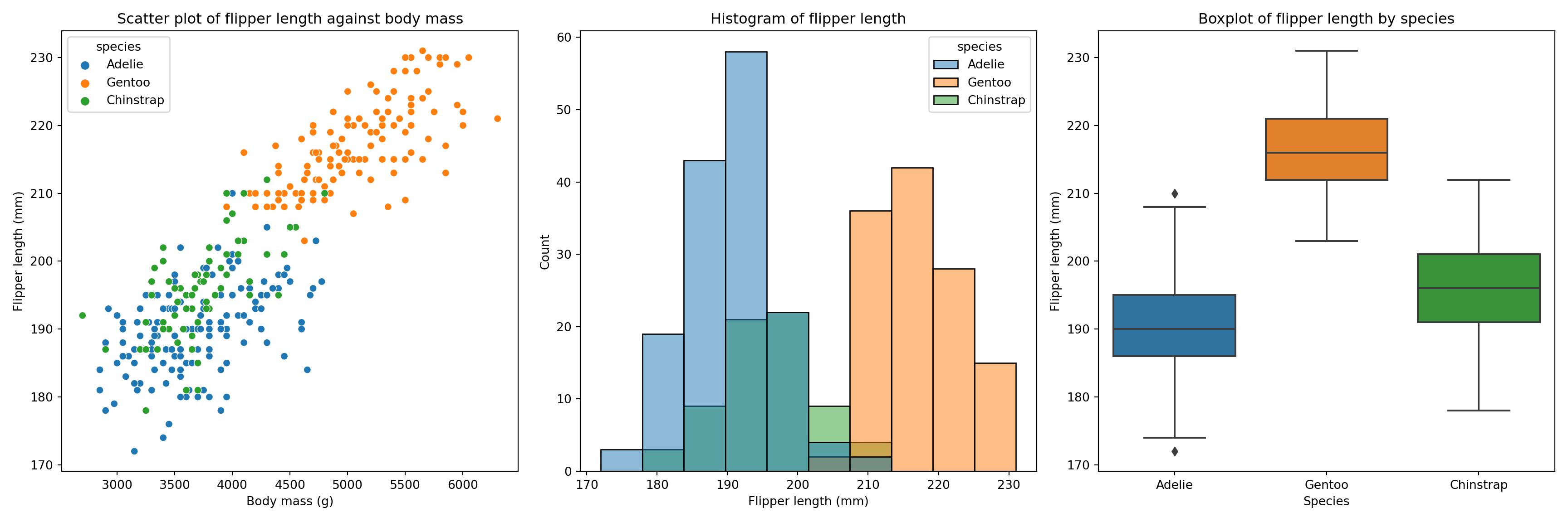
# Boxplot on the third subplot
sns.boxplot(data=penguins, # Set data
x="species", # Set x-axis variable
y="flipper_length_mm", # Set y-axis variable
ax=ax3) # Add plot to third subplot
# Add title and axis labels
ax3.set_title("Boxplot of flipper length by species") # Add title
ax3.set_xlabel("Species") # Add x-axis label
ax3.set_ylabel("Flipper length (mm)") # Add y-axis label
# Adjusts the subplots to fit into the figure area
plt.tight_layout()
# Show the plots
plt.show()